BAD DAY 2: ANOVA
1. Analysis of variance: ANOVA models
# Setting the right working dir

bad2dir = getwd()
setwd(bad2dir)
Loading the data: in this case we ae going to work with the growth1 data set
provided as art of this course. The data is contained within a .csv file.
# data=read.delim('./Data/growth.txt',header=TRUE)
data1 = read.csv('./Data/growth1.csv')
Let’s first have a look at the dimension of the data
dim(data1)- 31
- 2
Printing the column names:
colnames(data1)- 'Growth'
- 'Treatment'
Getting a basic statistical summary on the data:
summary(data1) Growth Treatment
Min. : 5.00 A :7
1st Qu.:14.00 B :5
Median :36.00 C :5
Mean :38.68 Control:4
3rd Qu.:61.50 D :5
Max. :83.00 E :5
# making the objects in the dataframe accessible
attach(data1)Treatment- C
- C
- C
- C
- C
- E
- E
- E
- E
- E
- D
- D
- D
- D
- D
- A
- A
- A
- A
- A
- A
- A
- B
- B
- B
- B
- B
- Control
- Control
- Control
- Control
In this case we have a column for the DEPENDENT variable (Growth) and a column for the FACTOR (Treatment).
The first column contains numeric data but the second contains letters. It does not matter to R which form you have your dependent factors (letters or numbers) but it will be easier to interpret the results if you use meaningful names.
Ready to run the analysis.
data.aov = aov(Growth ~ Treatment)Notice here the symbol (a tilde) in the model. This means take Growth as the DEPENDENT variable, indeed it depends on the Treatment.
We can then print the results of the analysis of variance
#see the results: not very clear
data.aov
Call:
aov(formula = Growth ~ Treatment)
Terms:
Treatment Residuals
Sum of Squares 19459.167 973.607
Deg. of Freedom 5 25
Residual standard error: 6.240536
Estimated effects may be unbalanced
In order to get more information we need to view the analysis summary:
summary(data.aov) Df Sum Sq Mean Sq F value Pr(>F)
Treatment 5 19459 3892 99.93 1.07e-15 ***
Residuals 25 974 39
---
Signif. codes: 0 ‘***’ 0.001 ‘**’ 0.01 ‘*’ 0.05 ‘.’ 0.1 ‘ ’ 1
2. Post-hoc testing
This was an example of a simple one-way anova. According to the summary we see that there is a significant effect of Treatment upon Growth. However, there are 5 treatments!
It is crucial to know which of these treatments are significantly different from the each other (e.g. control treatments). R provides a simple function to carry out the Tukey HSD test.
TukeyHSD(data.aov) Tukey multiple comparisons of means
95% family-wise confidence level
Fit: aov(formula = Growth ~ Treatment)
$Treatment
diff lwr upr p adj
B-A -12.65714 -23.918244 -1.396042 0.0211539
C-A 47.54286 36.281756 58.803958 0.0000000
Control-A -18.10714 -30.161431 -6.052855 0.0012274
D-A 32.94286 21.681756 44.203958 0.0000000
E-A 38.54286 27.281756 49.803958 0.0000000
C-B 60.20000 48.036621 72.363379 0.0000000
Control-B -5.45000 -18.351212 7.451212 0.7812490
D-B 45.60000 33.436621 57.763379 0.0000000
E-B 51.20000 39.036621 63.363379 0.0000000
Control-C -65.65000 -78.551212 -52.748788 0.0000000
D-C -14.60000 -26.763379 -2.436621 0.0121584
E-C -9.00000 -21.163379 3.163379 0.2390481
D-Control 51.05000 38.148788 63.951212 0.0000000
E-Control 56.65000 43.748788 69.551212 0.0000000
E-D 5.60000 -6.563379 17.763379 0.7157067
3. Two way ANOVA
Loading the data to be used
data2 = read.csv('./Data/growth2.csv')
names(data2)- 'Growth'
- 'Treatment'
- 'Gender'
detach(data1)  # detach the previoulsy attached data set
attach(data2) # making data2 accessibleGender- M
- M
- M
- F
- F
- F
- F
- M
- M
- M
- F
- F
- F
- M
- M
- M
- F
- F
- M
- M
- M
- F
- F
- F
- M
- M
- M
- F
- F
- M
- M
- F
- F
- M
- M
Treatment- C
- C
- C
- C
- C
- E
- E
- E
- E
- E
- D
- D
- D
- D
- D
- A
- A
- A
- A
- A
- A
- A
- B
- B
- B
- B
- B
- Control
- Control
- Control
- Control
- Control
- Control
- Control
- Control
length(Gender)35
We can compare the two times or the two shoes by looking at summary statistics or at parallel boxplots. To get the means for each level of each factor, use R’s tapply command.
This takes three arguments: the data you wish to summarize, the factor that determines the groups, and the function you wish to apply to each of the groups.
First we will compute the mean Growth as a function of the Treatment type:
tapply(Growth, Treatment, mean)- A
- 23.8571428571429
- B
- 11.2
- C
- 71.4
- Control
- 6
- D
- 56.8
- E
- 62.4
boxplot(Growth ~ Treatment, col = (1:6), ylab = 'Growth',
       xlab =  'Treatment')
Now we will compute the mean growth as a function of age:
tapply(Growth, Gender, mean)- F
- 36.5625
- M
- 33.6315789473684
boxplot(Growth ~ Gender, col = c('lightblue2', 'mediumpurple'), xlab = 'Gender',
        ylab = 'Growth')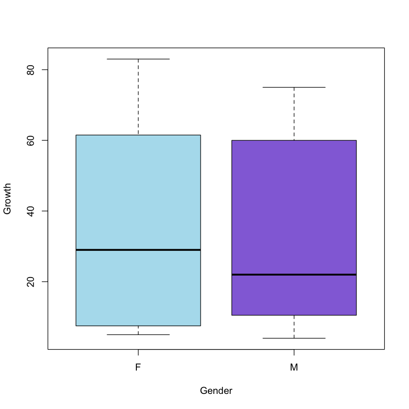
Comparing the two sets of means, we could draw the following preliminary conclusions:
- Females grow more
- The most effective treatment is E
But that could just be due to natural variability. We can check if this is the case by using a two way ANOVA analysis.
We prefer to start with a model taking into account the interaction between Gender and Treatment:
int <- aov(Growth ~ Gender * Treatment)
summary(int)
Df Sum Sq Mean Sq F value Pr(>F)
Gender 1 75 75 2.272 0.145
Treatment 5 23208 4642 141.340 <2e-16 ***
Gender:Treatment 5 129 26 0.783 0.572
Residuals 23 755 33
---
Signif. codes: 0 ‘***’ 0.001 ‘**’ 0.01 ‘*’ 0.05 ‘.’ 0.1 ‘ ’ 1
The p-value for the interaction term is $»0.05$ (not significant). This suggests we do not have to worry about their interaction!
So we repeat the process using a simple additive model.
noint <- aov(Growth ~ Gender + Treatment)
summary(noint)
Df Sum Sq Mean Sq F value Pr(>F)
Gender 1 75 75 2.364 0.135
Treatment 5 23208 4642 147.041 <2e-16 ***
Residuals 28 884 32
---
Signif. codes: 0 ‘***’ 0.001 ‘**’ 0.01 ‘*’ 0.05 ‘.’ 0.1 ‘ ’ 1
As you can see p-values for the Gender variable is quite large, suggesting that any effect we saw could well have been due to chance!
4. N-way analysis of variance
This example will use the dataset npk(Nitrogen - N, Phosphate - P, Potassium -
K) that is available in R with the MASS library (Modern Applied Statistics with
S)
library(MASS)npk
replications(yield ~ N * P * K, data = npk)| block | N | P | K | yield |
|---|---|---|---|---|
| 1 | 0 | 1 | 1 | 49.5 |
| 1 | 1 | 1 | 0 | 62.8 |
| 1 | 0 | 0 | 0 | 46.8 |
| 1 | 1 | 0 | 1 | 57.0 |
| 2 | 1 | 0 | 0 | 59.8 |
| 2 | 1 | 1 | 1 | 58.5 |
| 2 | 0 | 0 | 1 | 55.5 |
| 2 | 0 | 1 | 0 | 56.0 |
| 3 | 0 | 1 | 0 | 62.8 |
| 3 | 1 | 1 | 1 | 55.8 |
| 3 | 1 | 0 | 0 | 69.5 |
| 3 | 0 | 0 | 1 | 55.0 |
| 4 | 1 | 0 | 0 | 62.0 |
| 4 | 1 | 1 | 1 | 48.8 |
| 4 | 0 | 0 | 1 | 45.5 |
| 4 | 0 | 1 | 0 | 44.2 |
| 5 | 1 | 1 | 0 | 52.0 |
| 5 | 0 | 0 | 0 | 51.5 |
| 5 | 1 | 0 | 1 | 49.8 |
| 5 | 0 | 1 | 1 | 48.8 |
| 6 | 1 | 0 | 1 | 57.2 |
| 6 | 1 | 1 | 0 | 59.0 |
| 6 | 0 | 1 | 1 | 53.2 |
| 6 | 0 | 0 | 0 | 56.0 |
- N
- 12
- P
- 12
- K
- 12
- N:P
- 6
- N:K
- 6
- P:K
- 6
- N:P:K
- 3
#tapply
#?npkwith(npk, tapply(yield, list(N,P), mean))| 0 | 1 | |
|---|---|---|
| 0 | 51.71667 | 52.41667 |
| 1 | 59.21667 | 56.15000 |
with(npk, tapply(yield, list(N,K), mean))| 0 | 1 | |
|---|---|---|
| 0 | 52.88333 | 51.25000 |
| 1 | 60.85000 | 54.51667 |
with(npk, tapply(yield, list(P,K), mean))| 0 | 1 | |
|---|---|---|
| 0 | 57.60000 | 53.33333 |
| 1 | 56.13333 | 52.43333 |
npk.aov <- aov(yield ~ N * P * K, data = npk)TukeyHSD(npk.aov, conf.level=.99); Tukey multiple comparisons of means
99% family-wise confidence level
Fit: aov(formula = yield ~ N * P * K, data = npk)
$N
diff lwr upr p adj
1-0 5.616667 -0.9927112 12.22604 0.0245421
$P
diff lwr upr p adj
1-0 -1.183333 -7.792711 5.426044 0.6081875
$K
diff lwr upr p adj
1-0 -3.983333 -10.59271 2.626044 0.0974577
$`N:P`
diff lwr upr p adj
1:0-0:0 7.500000 -4.248642 19.248642 0.1294203
0:1-0:0 0.700000 -11.048642 12.448642 0.9961506
1:1-0:0 4.433333 -7.315308 16.181975 0.5257140
0:1-1:0 -6.800000 -18.548642 4.948642 0.1873570
1:1-1:0 -3.066667 -14.815308 8.681975 0.7743737
1:1-0:1 3.733333 -8.015308 15.481975 0.6554324
$`N:K`
diff lwr upr p adj
1:0-0:0 7.966667 -3.781975 19.715308 0.0999349
0:1-0:0 -1.633333 -13.381975 10.115308 0.9554188
1:1-0:0 1.633333 -10.115308 13.381975 0.9554188
0:1-1:0 -9.600000 -21.348642 2.148642 0.0382331
1:1-1:0 -6.333333 -18.081975 5.415308 0.2364506
1:1-0:1 3.266667 -8.481975 15.015308 0.7399770
$`P:K`
diff lwr upr p adj
1:0-0:0 -1.466667 -13.21531 10.281975 0.9670135
0:1-0:0 -4.266667 -16.01531 7.481975 0.5562955
1:1-0:0 -5.166667 -16.91531 6.581975 0.3986648
0:1-1:0 -2.800000 -14.54864 8.948642 0.8176375
1:1-1:0 -3.700000 -15.44864 8.048642 0.6615998
1:1-0:1 -0.900000 -12.64864 10.848642 0.9919305
$`N:P:K`
diff lwr upr p adj
1:0:0-0:0:0 12.33333333 -7.121667 31.788334 0.1841773
0:1:0-0:0:0 2.90000000 -16.555001 22.355001 0.9975401
1:1:0-0:0:0 6.50000000 -12.955001 25.955001 0.8280891
0:0:1-0:0:0 0.56666667 -18.888334 20.021667 1.0000000
1:0:1-0:0:0 3.23333333 -16.221667 22.688334 0.9952141
0:1:1-0:0:0 -0.93333333 -20.388334 18.521667 0.9999987
1:1:1-0:0:0 2.93333333 -16.521667 22.388334 0.9973597
0:1:0-1:0:0 -9.43333333 -28.888334 10.021667 0.4627120
1:1:0-1:0:0 -5.83333333 -25.288334 13.621667 0.8902999
0:0:1-1:0:0 -11.76666667 -31.221667 7.688334 0.2249895
1:0:1-1:0:0 -9.10000000 -28.555001 10.355001 0.5045183
0:1:1-1:0:0 -13.26666667 -32.721667 6.188334 0.1303264
1:1:1-1:0:0 -9.40000000 -28.855001 10.055001 0.4668300
1:1:0-0:1:0 3.60000000 -15.855001 23.055001 0.9909550
0:0:1-0:1:0 -2.33333333 -21.788334 17.121667 0.9993808
1:0:1-0:1:0 0.33333333 -19.121667 19.788334 1.0000000
0:1:1-0:1:0 -3.83333333 -23.288334 15.621667 0.9870208
1:1:1-0:1:0 0.03333333 -19.421667 19.488334 1.0000000
0:0:1-1:1:0 -5.93333333 -25.388334 13.521667 0.8819049
1:0:1-1:1:0 -3.26666667 -22.721667 16.188334 0.9949094
0:1:1-1:1:0 -7.43333333 -26.888334 12.021667 0.7204567
1:1:1-1:1:0 -3.56666667 -23.021667 15.888334 0.9914323
1:0:1-0:0:1 2.66666667 -16.788334 22.121667 0.9985452
0:1:1-0:0:1 -1.50000000 -20.955001 17.955001 0.9999671
1:1:1-0:0:1 2.36666667 -17.088334 21.821667 0.9993214
0:1:1-1:0:1 -4.16666667 -23.621667 15.288334 0.9793323
1:1:1-1:0:1 -0.30000000 -19.755001 19.155001 1.0000000
1:1:1-0:1:1 3.86666667 -15.588334 23.321667 0.9863677
# Now plotting the results
plot(TukeyHSD(npk.aov, conf.level=.99))


summary(npk.aov) Df Sum Sq Mean Sq F value Pr(>F)
N 1 189.3 189.28 6.161 0.0245 *
P 1 8.4 8.40 0.273 0.6082
K 1 95.2 95.20 3.099 0.0975 .
N:P 1 21.3 21.28 0.693 0.4175
N:K 1 33.1 33.14 1.078 0.3145
P:K 1 0.5 0.48 0.016 0.9019
N:P:K 1 37.0 37.00 1.204 0.2887
Residuals 16 491.6 30.72
---
Signif. codes: 0 ‘***’ 0.001 ‘**’ 0.01 ‘*’ 0.05 ‘.’ 0.1 ‘ ’ 1
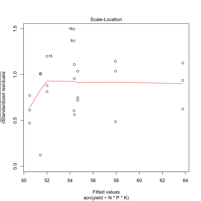
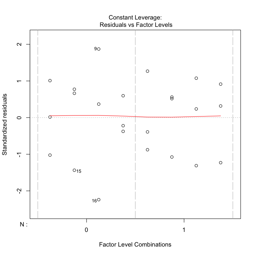
5. Final Diagnostic
- Is an ANOVA analysis appropriate?
- Are the basics assumptions met?
We should test for normality of data and homogeneity of variance.
-
The Normal distribution can be tested by using a Q-Q plot: if the points follow Q-Q line then data follow a normal distribution!
-
Shapiro-Wilk test for normality tests a null hypothesis of normal data.
-
The homogeneity of variance can be determined using the Bartlett Test of Homogeneity or Fligner-Killeen test of homogeneity of variances
plot(npk.aov)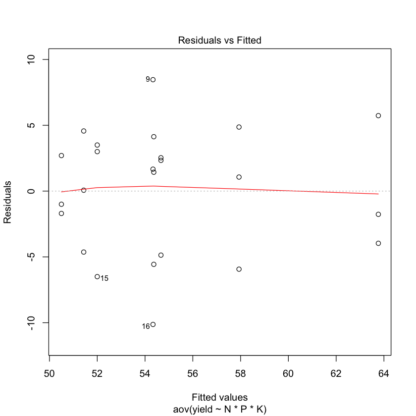

#plot.design(yield~N*P*K, data=npk);
#qqnorm(npk$yield); qqline(npk$yield, col=4)plot.design(yield~N*P*K, data = npk);
qqnorm(npk$yield);
qqline(npk$yield, col = 'mediumpurple', lwd = 3)

by(npk$yield, npk$N, shapiro.test);
by(npk$yield, npk$P, shapiro.test);
by(npk$yield, npk$K, shapiro.test)
npk$N: 0
Shapiro-Wilk normality test
data: dd[x, ]
W = 0.95781, p-value = 0.7522
------------------------------------------------------------
npk$N: 1
Shapiro-Wilk normality test
data: dd[x, ]
W = 0.96418, p-value = 0.8414
npk$P: 0
Shapiro-Wilk normality test
data: dd[x, ]
W = 0.96288, p-value = 0.824
------------------------------------------------------------
npk$P: 1
Shapiro-Wilk normality test
data: dd[x, ]
W = 0.95736, p-value = 0.7456
npk$K: 0
Shapiro-Wilk normality test
data: dd[x, ]
W = 0.97207, p-value = 0.9313
------------------------------------------------------------
npk$K: 1
Shapiro-Wilk normality test
data: dd[x, ]
W = 0.91886, p-value = 0.2766
bartlett.test(npk$yield ~ npk$N)
bartlett.test(npk$yield ~ npk$P)
bartlett.test(npk$yield ~ npk$K)
Bartlett test of homogeneity of variances
data: npk$yield by npk$N
Bartlett's K-squared = 0.057652, df = 1, p-value = 0.8102
Bartlett test of homogeneity of variances
data: npk$yield by npk$P
Bartlett's K-squared = 0.1555, df = 1, p-value = 0.6933
Bartlett test of homogeneity of variances
data: npk$yield by npk$K
Bartlett's K-squared = 3.0059, df = 1, p-value = 0.08296
fligner.test(npk$yield ~ npk$N);
fligner.test(npk$yield ~ npk$P);
fligner.test(npk$yield ~ npk$K);
Fligner-Killeen test of homogeneity of variances
data: npk$yield by npk$N
Fligner-Killeen:med chi-squared = 0.010063, df = 1, p-value = 0.9201
Fligner-Killeen test of homogeneity of variances
data: npk$yield by npk$P
Fligner-Killeen:med chi-squared = 0.0070479, df = 1, p-value = 0.9331
Fligner-Killeen test of homogeneity of variances
data: npk$yield by npk$K
Fligner-Killeen:med chi-squared = 2.6046, df = 1, p-value = 0.1066