BAD Day 1: Multiple hypothesis testing on Golub

In this tutorial we will do multiple hypothesis testing on the previsouly studied Golub data set.

Null Hypothesis $H_0$: states the assumption to be tested. We begin by assuming that the null Hypothesis is True
Alternative Hypothesis $H_1$: is the opposite of the null hypothesis

1. Loading the dataset

In [1]:

require(multtest)
data(golub)

Gene expression data (3051 genes and 38 tumor mRNA samples) from the leukemia microarray study of Golub et al. (1999). Pre-processing was done as described in Dudoit et al. (2002). The R code for pre-processing is available in the file ../doc/golub.R.

In [2]:

golub.expr<-golub
row.names(golub.expr)=golub.gnames[,3]

Numeric vector indicating the tumor class, 27 acute lymphoblastic leukemia (ALL) cases (code 0) and 11 acute myeloid leukemia (AML) cases (code 1).

In [3]:

colnames(golub.expr)= golub.cl

Setting the sample sizes

In [4]:

n.ALL <- 27
n.AML <- 11
cancer.type <- c(rep("ALL", n.ALL), rep("AML", n.AML))

Adding the cancer type to the column name, for the display

In [5]:

colnames(golub.expr) <-cancer.type

2. t.test with a single gene

In [6]:

g <- 347

Alternatively, you can select a gene randomly

In [7]:

## g <- sample(1:nrow(golub.expr),1)
g.profile <- as.vector(as.matrix(golub.expr[g,]))

Draw a barplot wiht color-coded cancer type

In [9]:

plot.col <- c('ALL'='mediumpurple', 'AML'='midnightblue')

barplot(g.profile, main = paste("Golub (1999), gene", g),
        col = plot.col[cancer.type], border = 'white')

legend('topright', c("ALL","AML"),col = plot.col[c("ALL","AML")],
       pch = 15, bty = "o")
box()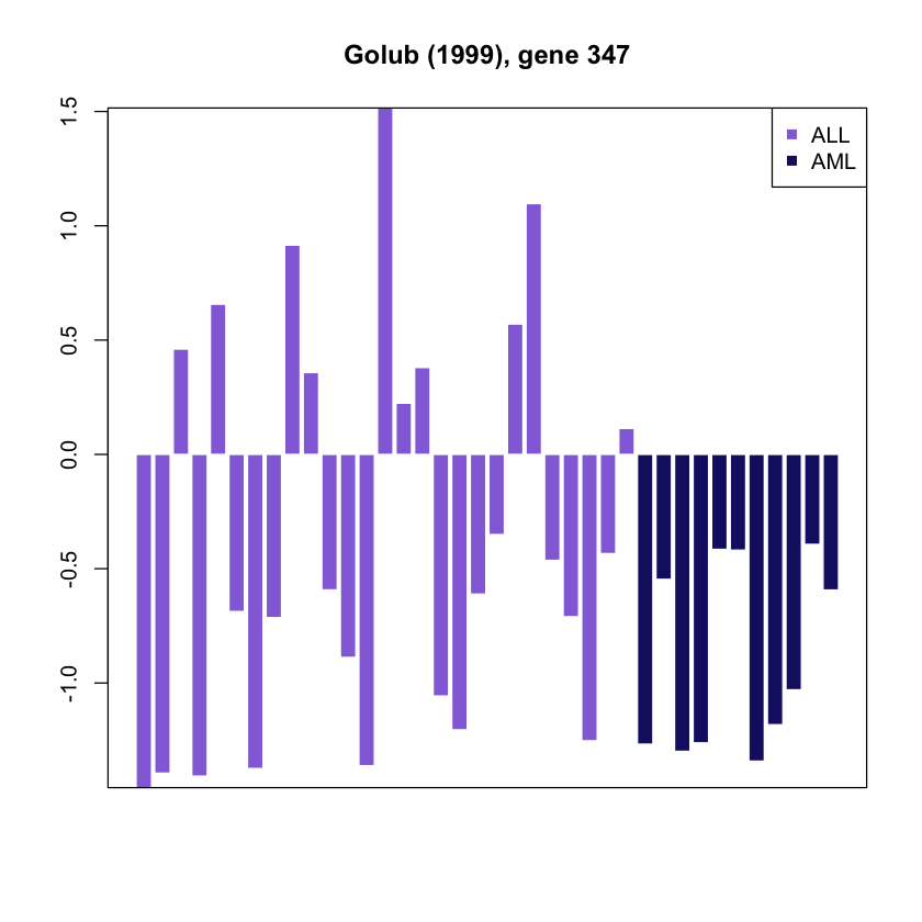

png

Separate data in two vectors

In [10]:

sample.ALL <- g.profile[cancer.type=="ALL"]
sample.AML <- g.profile[cancer.type=="AML"]

Compute manually the t test paramenters (not necessary, just to practice!)

Estimate the population means

In [11]:

mean.est.ALL <- mean(sample.ALL)
mean.est.AML <- mean(sample.AML)

Compute the sample sd

Remember the sd( ) function automatically computes the estimate corrected with sqrt(n-1)

In [12]:

sample.sd.ALL <- sd(sample.ALL) * sqrt((n.ALL-1)/n.ALL)
sample.sd.AML <- sd(sample.AML) * sqrt((n.AML-1)/n.AML)

Estimate the population standard deviation

In [13]:

sd.est.ALL <- sd(sample.ALL)
sd.est.AML <- sd(sample.AML)

Estimate the standard errors on the mean

In [14]:

sd.err.est.ALL <- sd(sample.ALL) / sqrt(n.ALL)
sd.err.est.AML <- sd(sample.AML) / sqrt(n.AML)

Estimate the standard deviation of the difference between the two means according to Student’s formula

In [15]:

diff.sd.est <- sqrt((n.ALL*sample.sd.ALL^2 + n.AML*sample.sd.AML^2) * (1/n.ALL + 1/n.AML) /(n.ALL+n.AML-2))

Compute t.obs

In [16]:

d <- abs(mean.est.ALL - mean.est.AML)
t.obs.Student <- d/diff.sd.est

Compute the P- vale. Since we are performing the two-tail test, the single-tail probability has to be multiplied by 3 in order to obtai the alpha risk

In [17]:

P.val.Student <- 2 * pt(q = t.obs.Student, df = n.ALL + n.AML-2, lower.tail = F)

This is what you should be doing… FAST!

3. Apply the Student-Fischer t-test

Note: this assumes that the two populations have equal variance.

In [18]:

t.student <- t.test(sample.ALL,sample.AML, var.equal=TRUE)
print(t.student)

4. Apply the Welch t-test

Note: this does not assume that the two populations have equal variance.

In [19]:

t.welch <- t.test(sample.ALL,sample.AML, var.equal=FALSE)
print(t.welch)

We want to test all the genes, so we could just loop over what was written before … (note it can take some time)

In [20]:

t.statistics <- vector()
P.values <- vector()
for (g in 1:nrow(golub.expr)) {
  #  print(paste("Testing gene", g))
  g.profile <- as.vector(golub.expr[g,])
  sample.ALL <- g.profile[cancer.type=="ALL"]
  sample.AML <- g.profile[cancer.type=="AML"]
  t <- t.test(sample.ALL,sample.AML)
  t.statistics <- append(t.statistics, t$statistic)
  P.values <- append(P.values, t$p.value)
}

In [21]:

 print(P.values)

For a more efficient way, you can use apply instead (not shown here)

In [22]:

Data=cbind(golub.expr,P.values)
colnames(Data)[39]='Raw.p'

Order data by pvalue

In [23]:

Data = Data[order(Data[,'Raw.p']),]

Perform p-value adjustments and add to the data frame

In [24]:

Datadf <- as.data.frame(Data)

In [25]:

Datadf$Bonferroni =
  p.adjust(Datadf$Raw.p,
           method = "bonferroni")

Datadf$BH =
  p.adjust(Datadf$Raw.p,
           method = "BH")

Datadf$Holm =
  p.adjust(Datadf$ Raw.p,
           method = "holm")

Datadf$Hochberg =
  p.adjust(Datadf$ Raw.p,
           method = "hochberg")

Datadf$Hommel =
  p.adjust(Datadf$ Raw.p,
           method = "hommel")

Datadf$BY =
  p.adjust(Datadf$ Raw.p,
           method = "BY")

5. Plotting the obtained data

In [26]:

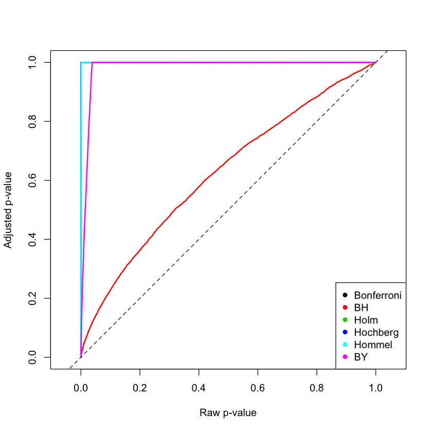
X = Datadf$Raw.p
Y = cbind(Datadf$Bonferroni,
          Datadf$BH,
          Datadf$Holm,
          Datadf$Hochberg,
          Datadf$Hommel,
          Datadf$BY)

In [27]:

matplot(X, Y,
        xlab="Raw p-value",
        ylab="Adjusted p-value",
        type="l",
        asp=1,
        col=1:6,
        lty=1,
        lwd=2)

legend('bottomright',
       legend = c("Bonferroni", "BH", "Holm", "Hochberg", "Hommel", "BY"),
       col = 1:6,
       cex = 1,    
       pch = 16)

abline(0, 1,
       col=1,
       lty=2,
       lwd=1)

png