BAD Day 1 : T-test
1. Loading the data set
require(multtest)
data(golub)
We will be usig the Gene Expression dataset from Golub et al (1999).
Gene expression data (3051 genes and 38 tumor mRNA samples) from the leukemia microarray study of Golub et al. (1999). Pre-processing was done as described in Dudoit et al. (2002). The R code for pre-processing is available in the file ../doc/golub.R. Source: Golub et al. (1999). Molecular classification of cancer: class discovery and class prediction by gene expression monitoring, Science, Vol. 286:531-537 (http://www-genome.wi.mit.edu/MPR/) .
golub.expr <- golub

# preliminar view of the data
head(golub.expr)| -1.45769 | -1.39420 | -1.42779 | -1.40715 | -1.42668 | -1.21719 | -1.37386 | -1.36832 | -1.47649 | -1.21583 | ⋯ | -1.08902 | -1.29865 | -1.26183 | -1.44434 | 1.10147 | -1.34158 | -1.22961 | -0.75919 | 0.84905 | -0.66465 |
| -0.75161 | -1.26278 | -0.09052 | -0.99596 | -1.24245 | -0.69242 | -1.37386 | -0.50803 | -1.04533 | -0.81257 | ⋯ | -1.08902 | -1.05094 | -1.26183 | -1.25918 | 0.97813 | -0.79357 | -1.22961 | -0.71792 | 0.45127 | -0.45804 |
| 0.45695 | -0.09654 | 0.90325 | -0.07194 | 0.03232 | 0.09713 | -0.11978 | 0.23381 | 0.23987 | 0.44201 | ⋯ | -0.43377 | -0.10823 | -0.29385 | 0.05067 | 1.69430 | -0.12472 | 0.04609 | 0.24347 | 0.90774 | 0.46509 |
| 3.13533 | 0.21415 | 2.08754 | 2.23467 | 0.93811 | 2.24089 | 3.36576 | 1.97859 | 2.66468 | -1.21583 | ⋯ | 0.29598 | -1.29865 | 2.76869 | 2.08960 | 0.70003 | 0.13854 | 1.75908 | 0.06151 | 1.30297 | 0.58186 |
| 2.76569 | -1.27045 | 1.60433 | 1.53182 | 1.63728 | 1.85697 | 3.01847 | 1.12853 | 2.17016 | -1.21583 | ⋯ | -1.08902 | -1.29865 | 2.00518 | 1.17454 | -1.47218 | -1.34158 | 1.55086 | -1.18107 | 1.01596 | 0.15788 |
| 2.64342 | 1.01416 | 1.70477 | 1.63845 | -0.36075 | 1.73451 | 3.36576 | 0.96870 | 2.72368 | -1.21583 | ⋯ | -1.08902 | -1.29865 | 1.73780 | 0.89347 | -0.52883 | -1.22168 | 0.90832 | -1.39906 | 0.51266 | 1.36249 |
golub.names is a matrix containing the names of the 3051
genes contained in golub. The three columns correspond to:
index, ID and name
row.names(golub.expr) = golub.gnames[,3]golub.cl is a numeric vector indicating the tumor class, 27 acute
lymphoblastic leukemia (ALL) cases (code 0) and 11 acute myeloid leukemia (AML)
cases (code 1).
colnames(golub.expr) = golub.clNow we need to set the sample sizes
n.ALL <- 27
n.AML <- 11

cancer.type <- c(rep('ALL', n.ALL), rep('AML', n.AML))
Adding the cancer type to the column name, for the display
colnames(golub.expr) <- cancer.typehead(golub.expr)| ALL | ALL | ALL | ALL | ALL | ALL | ALL | ALL | ALL | ALL | ⋯ | AML | AML | AML | AML | AML | AML | AML | AML | AML | AML | |
|---|---|---|---|---|---|---|---|---|---|---|---|---|---|---|---|---|---|---|---|---|---|
| AFFX-HUMISGF3A/M97935_MA_at | -1.45769 | -1.39420 | -1.42779 | -1.40715 | -1.42668 | -1.21719 | -1.37386 | -1.36832 | -1.47649 | -1.21583 | ⋯ | -1.08902 | -1.29865 | -1.26183 | -1.44434 | 1.10147 | -1.34158 | -1.22961 | -0.75919 | 0.84905 | -0.66465 |
| AFFX-HUMISGF3A/M97935_MB_at | -0.75161 | -1.26278 | -0.09052 | -0.99596 | -1.24245 | -0.69242 | -1.37386 | -0.50803 | -1.04533 | -0.81257 | ⋯ | -1.08902 | -1.05094 | -1.26183 | -1.25918 | 0.97813 | -0.79357 | -1.22961 | -0.71792 | 0.45127 | -0.45804 |
| AFFX-HUMISGF3A/M97935_3_at | 0.45695 | -0.09654 | 0.90325 | -0.07194 | 0.03232 | 0.09713 | -0.11978 | 0.23381 | 0.23987 | 0.44201 | ⋯ | -0.43377 | -0.10823 | -0.29385 | 0.05067 | 1.69430 | -0.12472 | 0.04609 | 0.24347 | 0.90774 | 0.46509 |
| AFFX-HUMRGE/M10098_5_at | 3.13533 | 0.21415 | 2.08754 | 2.23467 | 0.93811 | 2.24089 | 3.36576 | 1.97859 | 2.66468 | -1.21583 | ⋯ | 0.29598 | -1.29865 | 2.76869 | 2.08960 | 0.70003 | 0.13854 | 1.75908 | 0.06151 | 1.30297 | 0.58186 |
| AFFX-HUMRGE/M10098_M_at | 2.76569 | -1.27045 | 1.60433 | 1.53182 | 1.63728 | 1.85697 | 3.01847 | 1.12853 | 2.17016 | -1.21583 | ⋯ | -1.08902 | -1.29865 | 2.00518 | 1.17454 | -1.47218 | -1.34158 | 1.55086 | -1.18107 | 1.01596 | 0.15788 |
| AFFX-HUMRGE/M10098_3_at | 2.64342 | 1.01416 | 1.70477 | 1.63845 | -0.36075 | 1.73451 | 3.36576 | 0.96870 | 2.72368 | -1.21583 | ⋯ | -1.08902 | -1.29865 | 1.73780 | 0.89347 | -0.52883 | -1.22168 | 0.90832 | -1.39906 | 0.51266 | 1.36249 |
2. t.test with a single gene (step-by-step)
We will select the gene 347 for this example
g <- 347Alternatively, you can select a gene randomly
# g <- sample(1:nrow(golub.expr),1)
g.profile <- as.vector(as.matrix(golub.expr[g,]))
Draw a barplot with color-coded cancer type
plot.col <- c('ALL'='midnightblue', 'AML'='mediumpurple')

barplot(g.profile, main=paste("Golub (1999), gene", g),
        col=plot.col[cancer.type])
legend('topright', c("ALL","AML"),col=plot.col[c("ALL","AML")],
       pch=15, bty="o", bg='white')
box()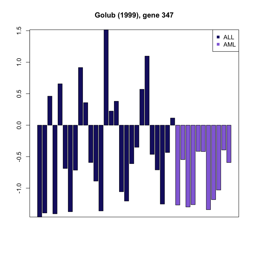
Separating the data in two vectors
sample.ALL <- g.profile[cancer.type=="ALL"]
sample.AML <- g.profile[cancer.type=="AML"]
Compute manually the t test parameters (not necessary, just to practice!)
Estimate the population means
mean.est.ALL <- mean(sample.ALL)
mean.est.AML <- mean(sample.AML)
Compute the sample standard deviations The sd() function automatically computes the estimate corrected with sqrt(n-1)
sample.sd.ALL <- sd(sample.ALL) * sqrt((n.ALL-1)/n.ALL)
sample.sd.AML <- sd(sample.AML) * sqrt((n.AML-1)/n.AML)
Estimate the population standard deviation
sd.est.ALL <- sd(sample.ALL)
sd.est.AML <- sd(sample.AML)
Estimate the standard deviations on the means
sd.err.est.ALL <- sd(sample.ALL) / sqrt(n.ALL)
sd.err.est.AML <- sd(sample.AML) / sqrt(n.AML)
Estimate the standard deviation of the difference between two means, according to Student’s formula
diff.sd.est <- sqrt((n.ALL*sample.sd.ALL^2 + n.AML*sample.sd.AML^2) * (1/n.ALL + 1/n.AML) /(n.ALL+n.AML-2))Compute t.obs
d <- abs(mean.est.ALL - mean.est.AML)
t.obs.Student <- d / diff.sd.est
Compute the P- vale. Since we are performing the two-tail test, the single-tail probability has to be multiplied by 3 in order to obtai the alpha risk
P.val.Student <- 2 * pt(q = t.obs.Student, df = n.ALL + n.AML-2, lower.tail = F)3. T-test the fast way
This is what you should be doing…
Suppose that the gene expression data from two groups of patients (experimental) are availabe and that the hypothesis is about the difference between the population means $\mu_1$ and $\mu_2$.
Thus $H_0: \mu_1 = \mu_2$ is to be tested against $H_0: \mu_1 \neq \mu_2$. If the gene expression data are $\left( x_1…x_n \right)$ and $\left(y_1…y_n\right)$ for the first and second group, respectively.
With the mean and variances of the first and the second groups being $\bar{x}$, $\bar{y}$ , $s_1^2$,$s_2^2$.
Then the t-statistic can be formulated as:
Note: the t-value is large if the difference between $\bar{x}$ and $\bar{y}$ is large and the standard deviations $s_1$ and $s_2$ are small. This corresponds to the Welch two-sample t-test.
3.2 Two-samples t-test with unequal variances (Welch t-test)
Golub et al. (1999) argue that gene CCND3 Cyclin D3 plays
an important role with respect to discriminating ALL from AML patients. We
previously generated the boxplots for this gene, which suggests that the ALL
population means differs from that of the AML. The null hypothesis of equal
means can be tested by using the appropriate factor and specification var.equal
= FALSE.
#t.test(sample.ALL,sample.AML, var.equal=FALSE)

# creating the gol.fac
gol.fac <-  factor(golub.cl, levels = 0:1, labels = c("AML", "ALL"))
t.test(golub[1042, ] ~ gol.fac, var.equal = FALSE)
Welch Two Sample t-test
data: golub[1042, ] by gol.fac
t = 6.3186, df = 16.118, p-value = 9.871e-06
alternative hypothesis: true difference in means is not equal to 0
95 percent confidence interval:
0.8363826 1.6802008
sample estimates:
mean in group AML mean in group ALL
1.8938826 0.6355909
The t value is significantly large, meaning that the two means differ largely with respect to the corresponding (standard error). As the p value is very small,the conclusion is to reject the null-hypothesis of equal means. The data provide strong evidence that the population means do differ.
3.1 Two-samples Student-Fischer t-test (samples with equal variances).
Suppose the same setup as in the above example. In this case, however, the variances $\sigma_1^2$ and $\sigma_2^2$ for the two groups are known to be equal. To test $H_0: \mu_1 = \mu_2$ against $H_1: \mu_1 \neq \mu_2$ there is a t-test which is based on the pooled sample variance $s_p^2$. The latter is defined by the weighted sum of the sample variances $s_1^2$ and $s_2^2$ e.g.
Then the t-value will be
The null hypothesis for gene CCND3 Cyclin D3 is that the mean of ALL differs from that of AML patients can be tested by the two-sample t-test using:
#t.test(sample.ALL,sample.AML, var.equal=TRUE)


t.test(golub[1042, ] ~ gol.fac, var.equal = TRUE)
Two Sample t-test
data: golub[1042, ] by gol.fac
t = 6.7983, df = 36, p-value = 6.046e-08
alternative hypothesis: true difference in means is not equal to 0
95 percent confidence interval:
0.8829143 1.6336690
sample estimates:
mean in group AML mean in group ALL
1.8938826 0.6355909
From the p-value $6.046 \times 10^{-8}$, the conclusion is to reject the null hypothesis of equal population means. Note that the p-value is slightly smaller than that of the previous test.