BAD DAY 2: Dimensionality reduction
1. PCA
(for more examples see http://manuals.bioinformatics.ucr.edu/home/R_BioCondManual )
Principal Component Analysis (PCA) is a data reduction technique that allows to simplify multidimensional data sets to a lower dimensional space ( tipically using 2 or 3 dimensions) for a first broad visual analysis of the data (via plotting and visual variance analysis).
The prcomp( ) and princomp( ) R functions are devoted to PCA.
The BioConductor library pcaMethods provides many additional PCA functions.
We are going to use the IRIS data set to demonstrate the use of PCA.
This data was used to show that these measurements could be used to differentiate between species of irises.
This data set contains the sepal/petal length and width measurements in centimeters for 50 flowers from each of 3 species of iris.
The Iris species are: setosa, versicolor, and virginica.
# Setting the working directory
bad2dir= getwd()
setwd(bad2dir)# Loading the data and getting a summary
data(iris)
str(iris);
summary(iris[1:4])
#dim(iris) Sepal.Length Sepal.Width Petal.Length Petal.Width
Min. :4.300 Min. :2.000 Min. :1.000 Min. :0.100
1st Qu.:5.100 1st Qu.:2.800 1st Qu.:1.600 1st Qu.:0.300
Median :5.800 Median :3.000 Median :4.350 Median :1.300
Mean :5.843 Mean :3.057 Mean :3.758 Mean :1.199
3rd Qu.:6.400 3rd Qu.:3.300 3rd Qu.:5.100 3rd Qu.:1.800
Max. :7.900 Max. :4.400 Max. :6.900 Max. :2.500
Now we will create a scatterplot of the dimensions against each other for the three species.
# Custom chosen colours
colours = c('steelblue3',  'mediumpurple', 'midnightblue')

# Plotting
pairs(iris[1:4], main = "Iris Data", pch = 19,
      col = colours[unclass(iris$Species)], labels = colnames(iris))


# adding legend
par(xpd=TRUE)
legend(x= 0.5, y = 0, levels(iris$Species), pt.bg = colours,
       pch = 21, bty = "n", ncol = 3)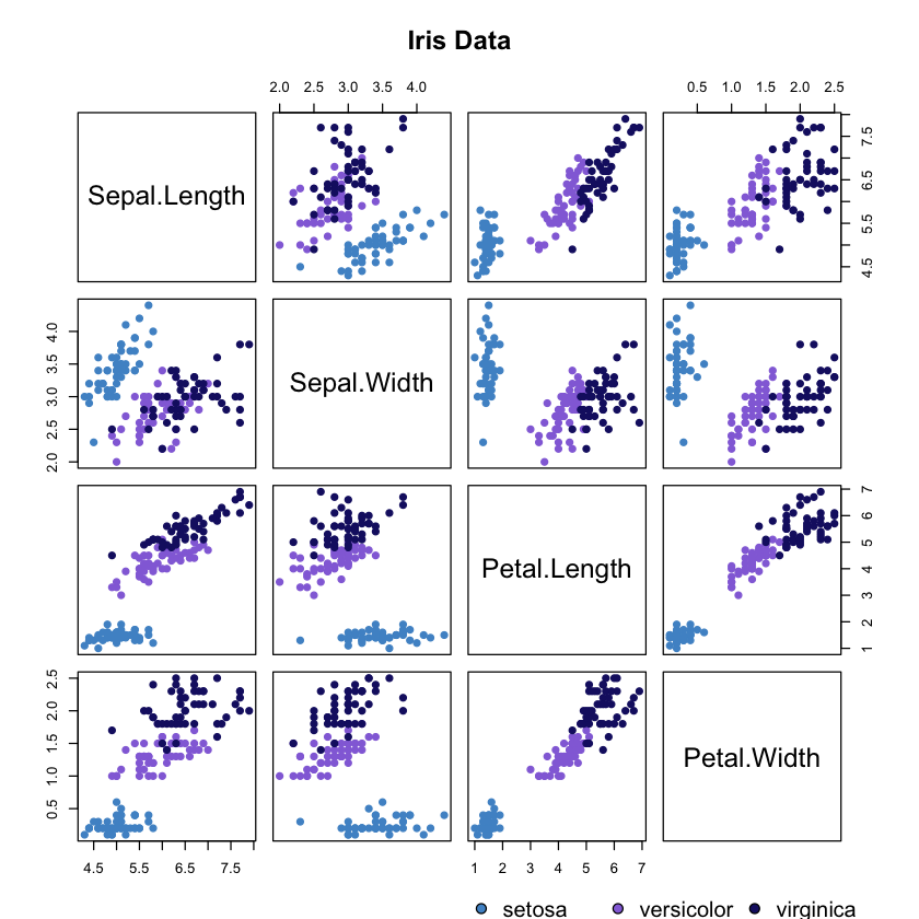
PCA is used to create linear combinations of the original data that capture as
much information in the original data as possible.
We will use the prcomp function.
-
If we work with standardized data (mean 0 std 1) we need to calculate the principal components through the correlation matrix.
-
If we work with raw data we need to calculate the principal components through the covariance matrix.
It is good practice to standardize our variables when these have different units and have very different variances. If they are in the same units either of the alteratives is appropriate.
In our example all variables are measured in centimetres but we will use the correlation matrix for simplicity’s sake.
First, we are going to examine the variability of all the numeric values
sapply(iris[1:4],var)- Sepal.Length
- 0.685693512304251
- Sepal.Width
- 0.189979418344519
- Petal.Length
- 3.11627785234899
- Petal.Width
- 0.581006263982103
range(sapply(iris[1:4],var))- 0.189979418344519
- 3.11627785234899
Maybe this range of variability is big in this context.
Thus, we will use the correlation matrix.
For this, we must standardize our variables using the scale() function:
iris.stand <- as.data.frame(scale(iris[,1:4]))
sapply(iris.stand,sd) #now, standard deviations are 1

#sapply(iris.stand,mean) #now, standard deviations are 1- Sepal.Length
- 1
- Sepal.Width
- 1
- Petal.Length
- 1
- Petal.Width
- 1
If we use the prcomp() function, we indicate scale=TRUE to use the
correlation matrix.
pca <- prcomp(iris.stand, scale = T)

#similar with princomp(): princomp(iris.stand, cor=T)
pca
Standard deviations:
[1] 1.7083611 0.9560494 0.3830886 0.1439265
Rotation:
PC1 PC2 PC3 PC4
Sepal.Length 0.5210659 -0.37741762 0.7195664 0.2612863
Sepal.Width -0.2693474 -0.92329566 -0.2443818 -0.1235096
Petal.Length 0.5804131 -0.02449161 -0.1421264 -0.8014492
Petal.Width 0.5648565 -0.06694199 -0.6342727 0.5235971
summary(pca)Importance of components:
PC1 PC2 PC3 PC4
Standard deviation 1.7084 0.9560 0.38309 0.14393
Proportion of Variance 0.7296 0.2285 0.03669 0.00518
Cumulative Proportion 0.7296 0.9581 0.99482 1.00000
This gives us the standard deviation of each component, and the proportion of
variance explained by each component.
The standard deviation is stored in (see str(pca)):
pca$sdev- 1.70836114932762
- 0.956049408486857
- 0.38308860015839
- 0.143926496617611
Usually the trend is to select up to 3 components (for visualization purposes) but we can have an indication on how many principal components should be retained.
Usually a scree plot helps making a decision. In R we can use the screeplot()
function:
#plot of variance of each PCA.
#It will be useful to decide how many principal components should be retained.
screeplot(pca, type = "lines", col = 'mediumpurple', lwd = 3)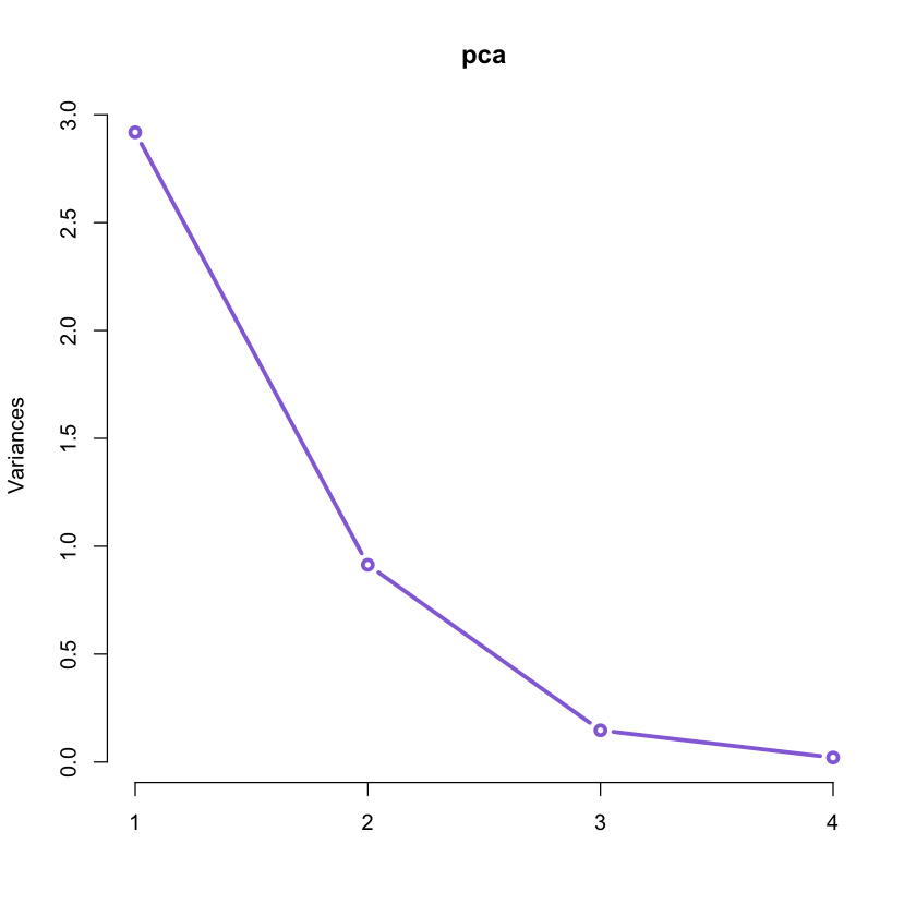
This plot together with the values of the Proportion of Variance and Cumulative
Proportion obtained by means of summary(pca) suggests that we can retain just
the first 2 components accounting for over 95% of the variation in the original
data!
#retreive loadings for the principal components:
pca$rotation # when using princomp(): pca$loadings| PC1 | PC2 | PC3 | PC4 | |
|---|---|---|---|---|
| Sepal.Length | 0.5210659 | -0.37741762 | 0.7195664 | 0.2612863 |
| Sepal.Width | -0.2693474 | -0.92329566 | -0.2443818 | -0.1235096 |
| Petal.Length | 0.5804131 | -0.02449161 | -0.1421264 | -0.8014492 |
| Petal.Width | 0.5648565 | -0.06694199 | -0.6342727 | 0.5235971 |
The weights of the PC1 are all similar but the one associated to Sepal.Width variable (it is negative). This one principal component accounts for over 72% of the variability in the data.
All weights on the second principal component are negative. Thus the PC2 might seem considered as an overall size measurement. This component explain the 23% of the variability.
The following figure show the first two components and the observations on the same diagram, which helps to interpret the factorial axes while looking at observations location.
The first component discriminate on one side the Sepal.Width and on the other side the rest of variables (see biplot). According to the second component, When the iris has larger sepal and petal values than average, the PC2 will be smaller than average.
unique(iris$Species)
as.numeric(unique(iris$Species))+1- setosa
- versicolor
- virginica
- 2
- 3
- 4
# biplot of first two principal components
biplot(pca, cex = 0.8)
abline(h = 0, v = 0, lty = 2, col = 8)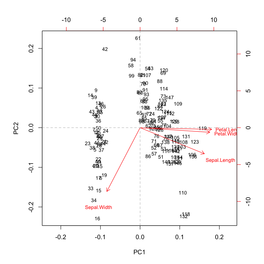
plot(pca$x, col = colours, pch = 19)

legend("topright", legend = unique(iris$Species), col = colours, pch= 19)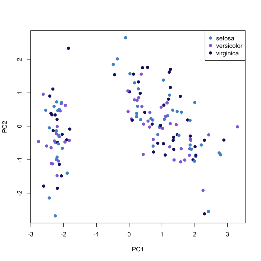
2. TSNE and comparison with PCA
The t-Distributed Stochastic Neighbor Embedding (t-SNE algorithm), by Laurens van der Maaten and Geoffrey Hinton, is a NON LINEAR dimensionality reduction algorithm. It enables the representation of high-dimensional data in two or three dimensions and allows visualization via scatter plots.
Barnes-Hut-SNE is a further improvement of the algorithm by Laurens van der Maaten, which uses Barnes-Hut approximations to significantly improve computational speed (O(N log N) instead of O(N2)). This makes it feasible to apply the algorithm to larger data sets.
We will follow the example proposed oh github <https://github.com/lmweber/Rtsne- example> using “Rtsne”, a package by Jesse Krijthe provides an R wrapper function for the C++ implementation of the Barnes-Hut-SNE algorithm.
The data set used in this example is the healthy human bone marrow data set
Marrow1.
# fist of all, just as an example, apply tsne on the IRIS dataset
library('Rtsne') # Load package
iris_unique <- unique(iris) # Remove duplicates
set.seed(42) # Sets seed for reproducibility
tsne_out <- Rtsne(as.matrix(iris_unique[,1:4])) # Run TSNE

plot(tsne_out$Y , col = colours, pch= 19) # Plot the result

legend("bottomright", legend = unique(iris$Species), col = colours, pch = 19)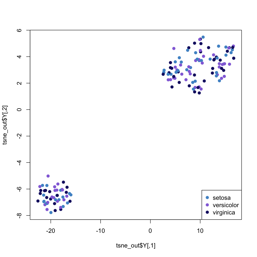
Here we will follow the example on GITHUB https://github.com/lmweber/Rtsne- example. The Marrow1 dataset is made of cells from different cell populations (types).
We will see how tsne will be able to group them as distinct clusters of points in the 2-dimensional projection. There is clear visual separation between clusters.
Amir et al. (2013) also independently verified the interpretation of the clusters using “manual gating” methods (visual inspection of 2-dimensional scatter plots), confirming that several clusters represent well-known cell types from immunology.
#install flowCore package from Bioconductor (to read FCS files)
source("https://bioconductor.org/biocLite.R")
biocLite("flowCore")

# install Rtsne package from CRAN (R implementation of Barnes-Hut-SNE algorithm)

#install.packages("Rtsne")

# load packages

library(flowCore)data <- exprs(read.FCS("./Rtsne-example-master/data/visne_marrow1.fcs", transformation = FALSE))
head(data)
unname(colnames(data)) # isotope and marker (protein) names| Event# | Time | Cell Length | 191-DNA | 193-DNA | 115-CD45 | 110,111,112,114-CD3 | 139-CD45RA | 141-pPLCgamma2 | 142-CD19 | ⋯ | 166-IkBalpha | 167-CD38 | 168-pH3 | 170-CD90 | 169-pP38 | 171-pBtk/Itk | 172-pS6 | 174-pSrcFK | 176-pCREB | 175-pCrkL |
|---|---|---|---|---|---|---|---|---|---|---|---|---|---|---|---|---|---|---|---|---|
| 22933 | 42448 | 14.39525 | 321.2244 | 434.9970 | 142.39886 | 18.5329704 | 117.579620 | 4.8356605 | 50.8025017 | ⋯ | 2.019981 | 32.1595116 | 14.3242693 | 8.78977966 | 53.843872 | 82.910294 | 6.8211913 | 5.774820 | 12.3001671 | 1.4769655 |
| 228744 | 667323 | 41.27012 | 209.3467 | 563.6180 | 50.66235 | 0.2076987 | 19.171650 | -1.3943130 | 10.0177841 | ⋯ | 4.779097 | -0.5546998 | 1.5282539 | -0.26177970 | 17.979921 | 1.054635 | 5.0797348 | 7.080018 | -1.7290312 | -1.0569905 |
| 230819 | 549730 | 28.91957 | 829.5733 | 1408.7177 | 503.61078 | 294.2422791 | 5.135233 | 0.8516778 | -0.1638297 | ⋯ | 12.946030 | 47.7583084 | 18.4628849 | 0.54432803 | 37.236912 | 38.177971 | 79.4033279 | 2.626387 | 23.7090988 | -1.4266791 |
| 131780 | 359184 | 26.11232 | 643.0649 | 992.3835 | 178.37289 | 359.2935181 | 79.340591 | -0.2172089 | 5.7050629 | ⋯ | 24.191151 | 49.7774315 | 5.1872330 | -0.07430215 | 6.879214 | 11.992647 | -0.2527083 | 9.006838 | -0.6766897 | -0.4470886 |
| 32212 | 56694 | 36.61685 | 713.0907 | 1131.0656 | 34.13390 | -12.1336746 | 1.377896 | 3.1527698 | -0.2193382 | ⋯ | 3.426270 | 42.7431793 | -0.8187979 | 9.73161793 | 10.562280 | 26.534126 | -0.7640409 | 50.811363 | 16.6444397 | 3.9240763 |
| 403958 | 834589 | 29.39848 | 638.0286 | 968.7856 | 288.91412 | 65.9604187 | 6.649710 | -0.7853550 | -1.4377729 | ⋯ | 1.359477 | 89.9450684 | 15.9464016 | 3.46092296 | 4.090930 | 51.456581 | 7.6963782 | 28.520178 | 5.2173581 | -0.3729125 |
- 'Event#'
- 'Time'
- 'Cell Length'
- '191-DNA'
- '193-DNA'
- '115-CD45'
- '110,111,112,114-CD3'
- '139-CD45RA'
- '141-pPLCgamma2'
- '142-CD19'
- '144-CD11b'
- '145-CD4'
- '146-CD8'
- '148-CD34'
- '150-pSTAT5'
- '147-CD20'
- '152-Ki67'
- '154-pSHP2'
- '151-pERK1/2'
- '153-pMAPKAPK2'
- '156-pZAP70/Syk'
- '158-CD33'
- '160-CD123'
- '159-pSTAT3'
- '164-pSLP-76'
- '165-pNFkB'
- '166-IkBalpha'
- '167-CD38'
- '168-pH3'
- '170-CD90'
- '169-pP38'
- '171-pBtk/Itk'
- '172-pS6'
- '174-pSrcFK'
- '176-pCREB'
- '175-pCrkL'
# select markers to use in calculation of t-SNE projection
# CD11b, CD123, CD19, CD20, CD3, CD33, CD34, CD38, CD4, CD45, CD45RA, CD8, CD90
# (see Amir et al. 2013, Supplementary Tables 1 and 2)

colnames_proj <- unname(colnames(data))[c(11, 23, 10, 16, 7, 22, 14, 28, 12, 6, 8, 13, 30)]
colnames_proj  # check carefully!


# arcsinh transformation
# (see Amir et al. 2013, Online Methods, "Processing of mass cytometry data")

asinh_scale <- 5
data <- asinh(data / asinh_scale)  # transforms all columns! including event number etc


# subsampling

nsub <- 10000
set.seed(123)  # set random seed
data <- data[sample(1:nrow(data), nsub), ]

dim(data)- '144-CD11b'
- '160-CD123'
- '142-CD19'
- '147-CD20'
- '110,111,112,114-CD3'
- '158-CD33'
- '148-CD34'
- '167-CD38'
- '145-CD4'
- '115-CD45'
- '139-CD45RA'
- '146-CD8'
- '170-CD90'
- 10000
- 36
# prepare data for Rtsne

data <- data[, colnames_proj]      # select columns to use
data <- data[!duplicated(data), ]  # remove rows containing duplicate values within rounding

dim(data)- 9902
- 13
# Exporting the subsample data in TXT format

file <- paste("./Rtsne-example-master/data/viSNE_Marrow1_nsub", nsub,".txt", sep = "")
write.table(data, file = file, row.names = FALSE, quote = FALSE, sep = "\t")
Running the Rtsne (Barnes-Hut_SNE algorithm) without PCA step (see Amir et al. 2013, Online Methods, “viSNE analysis”)
set.seed(123)  # set random seed
rtsne_out <- Rtsne(as.matrix(data), pca = FALSE, verbose = TRUE)# plot 2D t-SNE projection
# Uncomment the lines below if you want to save to a separate .PNG file
# file_plot <- paste("./Rtsne-example-master/plots/Rtsne_viSNE_Marrow1_nsub", nsub, ".png", sep = "")
# png(file_plot, width = 900, height = 900)
plot(rtsne_out$Y, asp =1, pch = 21, col = 'mediumpurple',
cex = 0.75, cex.axis = 1.25, cex.lab = 1.25, cex.main = 1.5,
xlab = "t-SNE dimension 1", ylab = "t-SNE dimension 2",
main = "2D t-SNE projection")
# Uncomment if saving to a pgn file
#dev(off)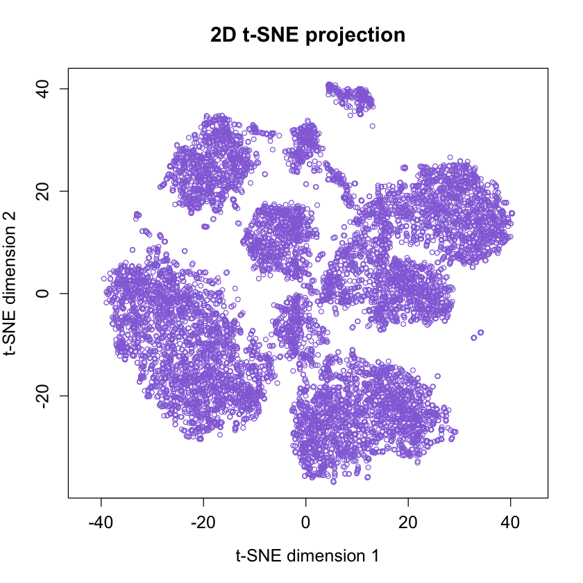
Compare to PCA
pca_data = princomp(as.matrix(data))$scores[,1:2]
plot(pca_data, col= 'steelblue3')

#text(pca_iris, labels=iris$Species,col=colors[iris$Species])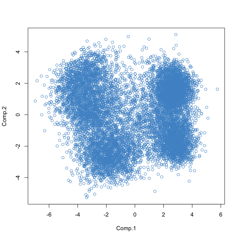
About the interpretation of TSNE
SOME EXAMPLES FROM https://gist.github.com/mikelove/74bbf5c41010ae1dc94281cface90d32 on the delicate interpretation of tsne when the underlyng structure of the data is LINEAR
Explore tsne on linear data. First install (if needed) and load the required packages.
library(rafalib)
library(RColorBrewer)
library(Rtsne)
library(tsne)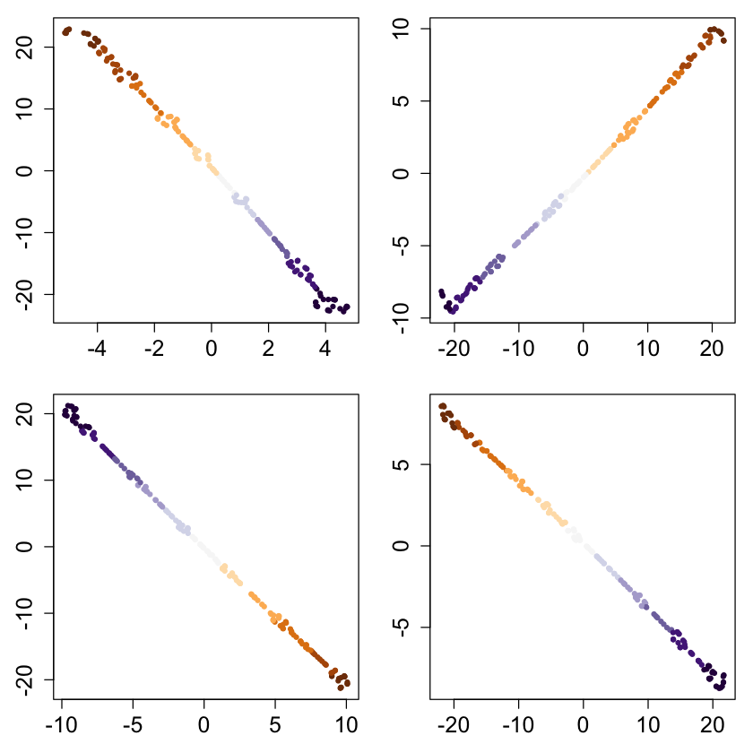
library(pracma)par(mfrow=c(1, 2))
for (i in 2:5) {
set.seed(i)
x <- runif(n, -1, 1)
cols <- brewer.pal(11, "PuOr")[as.integer(cut(x, 11))]
ortho <- randortho(m)
X <- cbind(x, matrix(0,ncol=m-1,nrow=n)) %*% ortho
res <- tsne(X)
plot(res, col=cols, pch=20, xlab="", ylab="", main="tsne")
res <- Rtsne(X)
plot(res$Y, col=cols, pch=20, xlab="", ylab="", main="Rtsne")
}Error in runif(n, -1, 1): object 'n' not found
Traceback:
1. runif(n, -1, 1) # at line 5 of file <text>
n <- 200
m <- 40
set.seed(1)
x <- runif(n, -1, 1)
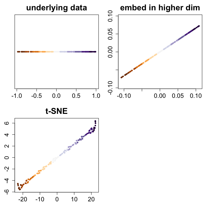
bigpar(2,2,mar=c(3,3,3,1))
cols <- brewer.pal(11, "PuOr")[as.integer(cut(x, 11))]
plot(x, rep(0,n), ylim=c(-1,1), yaxt="n", xlab="", ylab="",
col=cols, pch=20, main="underlying data")
ortho <- randortho(m)
X <- cbind(x, matrix(0,ncol=m-1,nrow=n)) %*% ortho
plot(X[,1:2], asp=1, col=cols, pch=20, xlab="", ylab="", main="embed in higher dim")
res <- tsne(X)
plot(res, col=cols, pch=20, xlab="", ylab="", main="t-SNE")
bigpar(2,2,mar=c(3,3,1,1))
for (i in 2:5) {
set.seed(i)
x <- runif(n, -1, 1)
cols <- brewer.pal(11, "PuOr")[as.integer(cut(x, 11))]
ortho <- randortho(m)
X <- cbind(x, matrix(0,ncol=m-1,nrow=n)) %*% ortho
res <- tsne(X);
plot(res, col=cols, pch=20, xlab="", ylab="")
}