BAD Day 1: Tutorial
0. Source/install the needed packages
In [1]:# In case you need to install the packages
install.packages("xlsx")
install.packages("gdata")
install.packages("ape")
source("http://bioconductor.org/biocLite.R");
biocLite("multtest");
1. Exploratory data analysis
We will be usig the Gene Expression dataset from Golub et al (1999). The
gene expression data collected by Golub et al. (1999) are among the most
classical in bioinformatics. A selection of the set is called golub which is
contained in the multtest package loaded before.
The data consist of gene expression values of 3051 genes (rows) from 38 leukemia patients Pre-processing was done as described in Dudoit et al. (2002). The R code for pre-processing is available in the file ../doc/golub.R.
Source: Golub et al. (1999). Molecular classification of cancer: class discovery and class prediction by gene expression monitoring, Science, Vol. 286:531-537. (http://www-genome.wi.mit.edu/MPR/).
In [3]:require(multtest);
# Usage
data(golub);
# If you need more information on the data set just
# uncomment the line below
# ?golub
Data set values:
golub: matrix of gene expression levels for the 38 tumor mRNA samples, rows correspond to genes (3051 genes) and columns to mRNA samples.golub.cl: numeric vector indicating the tumor class, 27 acute lymphoblastic leukemia (ALL) cases (code 0) and 11 acute myeloid leukemia (AML) cases (code 1).golub.names: a matrix containing the names of the 3051 genes for the expression matrix golub. The three columns correspond to the gene index, ID, and Name, respectively.
# Checking the dimension of the data
dim(golub)
- 3051
- 38
# we will have a look at the first rows contained in the data set
head(golub)
| -1.45769 | -1.39420 | -1.42779 | -1.40715 | -1.42668 | -1.21719 | -1.37386 | -1.36832 | -1.47649 | -1.21583 | ⋯ | -1.08902 | -1.29865 | -1.26183 | -1.44434 | 1.10147 | -1.34158 | -1.22961 | -0.75919 | 0.84905 | -0.66465 |
| -0.75161 | -1.26278 | -0.09052 | -0.99596 | -1.24245 | -0.69242 | -1.37386 | -0.50803 | -1.04533 | -0.81257 | ⋯ | -1.08902 | -1.05094 | -1.26183 | -1.25918 | 0.97813 | -0.79357 | -1.22961 | -0.71792 | 0.45127 | -0.45804 |
| 0.45695 | -0.09654 | 0.90325 | -0.07194 | 0.03232 | 0.09713 | -0.11978 | 0.23381 | 0.23987 | 0.44201 | ⋯ | -0.43377 | -0.10823 | -0.29385 | 0.05067 | 1.69430 | -0.12472 | 0.04609 | 0.24347 | 0.90774 | 0.46509 |
| 3.13533 | 0.21415 | 2.08754 | 2.23467 | 0.93811 | 2.24089 | 3.36576 | 1.97859 | 2.66468 | -1.21583 | ⋯ | 0.29598 | -1.29865 | 2.76869 | 2.08960 | 0.70003 | 0.13854 | 1.75908 | 0.06151 | 1.30297 | 0.58186 |
| 2.76569 | -1.27045 | 1.60433 | 1.53182 | 1.63728 | 1.85697 | 3.01847 | 1.12853 | 2.17016 | -1.21583 | ⋯ | -1.08902 | -1.29865 | 2.00518 | 1.17454 | -1.47218 | -1.34158 | 1.55086 | -1.18107 | 1.01596 | 0.15788 |
| 2.64342 | 1.01416 | 1.70477 | 1.63845 | -0.36075 | 1.73451 | 3.36576 | 0.96870 | 2.72368 | -1.21583 | ⋯ | -1.08902 | -1.29865 | 1.73780 | 0.89347 | -0.52883 | -1.22168 | 0.90832 | -1.39906 | 0.51266 | 1.36249 |
The gene names are collected in the matrix golub.gnames of which the columns
correspond to the gene index, ID, and Name, respectively.
# Adding 3051 gene names
row.names(golub) = golub.gnames[,3]

head(golub)
| AFFX-HUMISGF3A/M97935_MA_at | -1.45769 | -1.39420 | -1.42779 | -1.40715 | -1.42668 | -1.21719 | -1.37386 | -1.36832 | -1.47649 | -1.21583 | ⋯ | -1.08902 | -1.29865 | -1.26183 | -1.44434 | 1.10147 | -1.34158 | -1.22961 | -0.75919 | 0.84905 | -0.66465 |
|---|---|---|---|---|---|---|---|---|---|---|---|---|---|---|---|---|---|---|---|---|---|
| AFFX-HUMISGF3A/M97935_MB_at | -0.75161 | -1.26278 | -0.09052 | -0.99596 | -1.24245 | -0.69242 | -1.37386 | -0.50803 | -1.04533 | -0.81257 | ⋯ | -1.08902 | -1.05094 | -1.26183 | -1.25918 | 0.97813 | -0.79357 | -1.22961 | -0.71792 | 0.45127 | -0.45804 |
| AFFX-HUMISGF3A/M97935_3_at | 0.45695 | -0.09654 | 0.90325 | -0.07194 | 0.03232 | 0.09713 | -0.11978 | 0.23381 | 0.23987 | 0.44201 | ⋯ | -0.43377 | -0.10823 | -0.29385 | 0.05067 | 1.69430 | -0.12472 | 0.04609 | 0.24347 | 0.90774 | 0.46509 |
| AFFX-HUMRGE/M10098_5_at | 3.13533 | 0.21415 | 2.08754 | 2.23467 | 0.93811 | 2.24089 | 3.36576 | 1.97859 | 2.66468 | -1.21583 | ⋯ | 0.29598 | -1.29865 | 2.76869 | 2.08960 | 0.70003 | 0.13854 | 1.75908 | 0.06151 | 1.30297 | 0.58186 |
| AFFX-HUMRGE/M10098_M_at | 2.76569 | -1.27045 | 1.60433 | 1.53182 | 1.63728 | 1.85697 | 3.01847 | 1.12853 | 2.17016 | -1.21583 | ⋯ | -1.08902 | -1.29865 | 2.00518 | 1.17454 | -1.47218 | -1.34158 | 1.55086 | -1.18107 | 1.01596 | 0.15788 |
| AFFX-HUMRGE/M10098_3_at | 2.64342 | 1.01416 | 1.70477 | 1.63845 | -0.36075 | 1.73451 | 3.36576 | 0.96870 | 2.72368 | -1.21583 | ⋯ | -1.08902 | -1.29865 | 1.73780 | 0.89347 | -0.52883 | -1.22168 | 0.90832 | -1.39906 | 0.51266 | 1.36249 |
# Let's just have a look at the top 20 genes ID's contained in golub.gnames
head(golub.gnames[,2], n = 20)
- 'AFFX-HUMISGF3A/M97935_MA_at (endogenous control)'
- 'AFFX-HUMISGF3A/M97935_MB_at (endogenous control)'
- 'AFFX-HUMISGF3A/M97935_3_at (endogenous control)'
- 'AFFX-HUMRGE/M10098_5_at (endogenous control)'
- 'AFFX-HUMRGE/M10098_M_at (endogenous control)'
- 'AFFX-HUMRGE/M10098_3_at (endogenous control)'
- 'AFFX-HUMGAPDH/M33197_5_at (endogenous control)'
- 'AFFX-HUMGAPDH/M33197_M_at (endogenous control)'
- 'AFFX-HSAC07/X00351_5_at (endogenous control)'
- 'AFFX-HSAC07/X00351_M_at (endogenous control)'
- 'AFFX-HUMTFRR/M11507_5_at (endogenous control)'
- 'AFFX-HUMTFRR/M11507_M_at (endogenous control)'
- 'AFFX-HUMTFRR/M11507_3_at (endogenous control)'
- 'AFFX-M27830_5_at (endogenous control)'
- 'AFFX-M27830_M_at (endogenous control)'
- 'AFFX-M27830_3_at (endogenous control)'
- 'AFFX-HSAC07/X00351_3_st (endogenous control)'
- 'AFFX-HUMGAPDH/M33197_M_st (endogenous control)'
- 'AFFX-HUMGAPDH/M33197_3_st (endogenous control)'
- 'AFFX-HSAC07/X00351_M_st (endogenous control)'
Twenty-seven patients are diagnosed as acute lymphoblastic leukemia (ALL) and eleven as acute myeloid leukemia (AML). The tumor class is given by the numeric vector golub.cl, where ALL is indicated by 0 and AML by 1.
In [8]:colnames(golub) = golub.cl
head(golub)
| 0 | 0 | 0 | 0 | 0 | 0 | 0 | 0 | 0 | 0 | ⋯ | 1 | 1 | 1 | 1 | 1 | 1 | 1 | 1 | 1 | 1 | |
|---|---|---|---|---|---|---|---|---|---|---|---|---|---|---|---|---|---|---|---|---|---|
| AFFX-HUMISGF3A/M97935_MA_at | -1.45769 | -1.39420 | -1.42779 | -1.40715 | -1.42668 | -1.21719 | -1.37386 | -1.36832 | -1.47649 | -1.21583 | ⋯ | -1.08902 | -1.29865 | -1.26183 | -1.44434 | 1.10147 | -1.34158 | -1.22961 | -0.75919 | 0.84905 | -0.66465 |
| AFFX-HUMISGF3A/M97935_MB_at | -0.75161 | -1.26278 | -0.09052 | -0.99596 | -1.24245 | -0.69242 | -1.37386 | -0.50803 | -1.04533 | -0.81257 | ⋯ | -1.08902 | -1.05094 | -1.26183 | -1.25918 | 0.97813 | -0.79357 | -1.22961 | -0.71792 | 0.45127 | -0.45804 |
| AFFX-HUMISGF3A/M97935_3_at | 0.45695 | -0.09654 | 0.90325 | -0.07194 | 0.03232 | 0.09713 | -0.11978 | 0.23381 | 0.23987 | 0.44201 | ⋯ | -0.43377 | -0.10823 | -0.29385 | 0.05067 | 1.69430 | -0.12472 | 0.04609 | 0.24347 | 0.90774 | 0.46509 |
| AFFX-HUMRGE/M10098_5_at | 3.13533 | 0.21415 | 2.08754 | 2.23467 | 0.93811 | 2.24089 | 3.36576 | 1.97859 | 2.66468 | -1.21583 | ⋯ | 0.29598 | -1.29865 | 2.76869 | 2.08960 | 0.70003 | 0.13854 | 1.75908 | 0.06151 | 1.30297 | 0.58186 |
| AFFX-HUMRGE/M10098_M_at | 2.76569 | -1.27045 | 1.60433 | 1.53182 | 1.63728 | 1.85697 | 3.01847 | 1.12853 | 2.17016 | -1.21583 | ⋯ | -1.08902 | -1.29865 | 2.00518 | 1.17454 | -1.47218 | -1.34158 | 1.55086 | -1.18107 | 1.01596 | 0.15788 |
| AFFX-HUMRGE/M10098_3_at | 2.64342 | 1.01416 | 1.70477 | 1.63845 | -0.36075 | 1.73451 | 3.36576 | 0.96870 | 2.72368 | -1.21583 | ⋯ | -1.08902 | -1.29865 | 1.73780 | 0.89347 | -0.52883 | -1.22168 | 0.90832 | -1.39906 | 0.51266 | 1.36249 |
Note that sometimes it is better to construct a factor which indicates the tumor
class of the patients. Such a factor could be used for instance to separate the
tumor groups for plotting purposes. The factor (gol.fac) can be contructed as
follows.
gol.fac <- factor(golub.cl, levels = 0:1, labels = c("AML", "ALL"))
The labels correspond to the two tumor classes. The evaluation of gol.fac==”ALL” returns TRUE for the first twenty-seven values and FALSE for the remaining eleven, which is useful as a column index for selecting the expression values of the ALL patients. The expression values of gene CCND3 Cyclin D3 from the ALL patients can now be printed to the screen, as follows.
In [10]:golub[1042, gol.fac == "ALL"]
- 1
- 0.88941
- 1
- 1.45014
- 1
- 0.42904
- 1
- 0.82667
- 1
- 0.63637
- 1
- 1.0225
- 1
- 0.12758
- 1
- -0.74333
- 1
- 0.73784
- 1
- 0.4947
- 1
- 1.12058
Creating the exploratory plots
1.1. Plotting the value of gene (CCND3) in all nRNA samples (M92287_at)
We shall first have a look at the expression values of a gener with manufacurer
name M92278_at, which is known in biology as “CCND3 Cyclin D3”.
The expression values of this gene are collected in row 1042 of golub. To load the data and to obtain the relevant information from row 1042 of golub.gnames, use the following:
In [11]:mygene <- golub[1042, ]
The data has now been stored in the golub matrix. We will now plot the
expression values od the gene CCND3 Cyclin D3.
plot(mygene)
 In the previous plot we just used the default plotting preferences within R base
plotting.We can do some improvements so that the plot is easily understood.
In the previous plot we just used the default plotting preferences within R base
plotting.We can do some improvements so that the plot is easily understood.
plot(mygene, pch = 15, col = 'slateblue', ylab = 'Expression value of gene: CCND3',
    main = ' Gene expression values of CCND3 Cyclin D3')
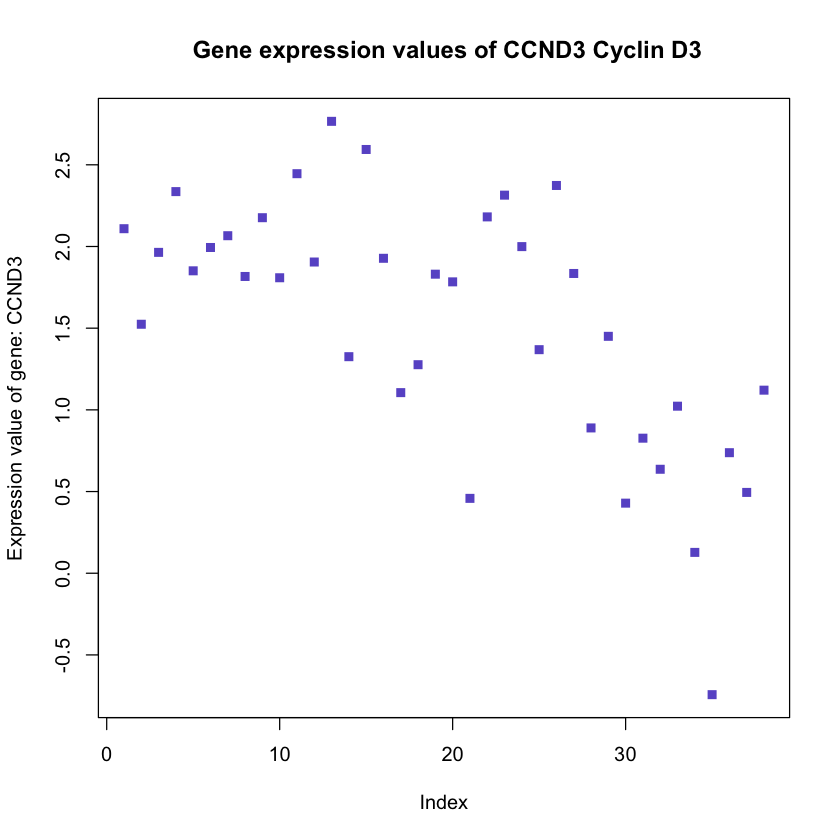 In this plot the vertical axis corresponds to the size of the expression values
and the horizontal axis the index of the patients.
In this plot the vertical axis corresponds to the size of the expression values
and the horizontal axis the index of the patients.
1.2. Gene expression between patient 1 (ALL) and patient 38 (AML)
In [14]:plot(golub[,1], golub[,38])
 Adding diagonal lines to the plot and changing axes labels
plot(golub[,1], golub[,38], xlab = 'Patient 1 (ALL)', ylab = 'Patient 38 (AML)')
abline(a = 0, b = 1, col = 'mediumpurple', lwd =3)

1.3. Scatter plots to detect independence
In [16]:mysamplist <- golub[, c(1:15)]
colnames(mysamplist) = c(1:15)
plot(as.data.frame(mysamplist), pch='.')

1.4. Bar plot of 4 cyclin genes expression values in 3 ALL and AML patients
We will analyse the expression values of the D13639_at, M92287_at, U11791_at,
Z36714_AT genes in three chosen AML and ALL patients
mygenelist <- golub[c(85, 1042, 1212, 2240), c(1:3, 36:38)]

# having a look at the data set chosen
mygenelist
| 0 | 0 | 0 | 1 | 1 | 1 | |
|---|---|---|---|---|---|---|
| D13639_at | 2.09511 | 1.71953 | -1.46227 | -0.92935 | -0.11091 | 1.15591 |
| M92287_at | 2.10892 | 1.52405 | 1.96403 | 0.73784 | 0.49470 | 1.12058 |
| U11791_at | -0.11439 | -0.72887 | -0.39674 | -0.94364 | 0.05047 | 0.05905 |
| Z36714_at | -1.45769 | -1.39420 | -1.46227 | -1.39906 | -1.34579 | -1.32403 |
barplot(mygenelist)
box()
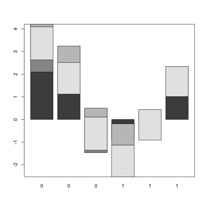 The plot is not very easy to read, so we will add some colours and a legend so
that we know which gene each bar segment corresponds to.
The plot is not very easy to read, so we will add some colours and a legend so
that we know which gene each bar segment corresponds to.
# custom colours
colours = c('lightblue2',   'slateblue', '#BD7BB8', '#2B377A')

barplot(mygenelist, col = colours, legend = TRUE, border = 'white')
box()
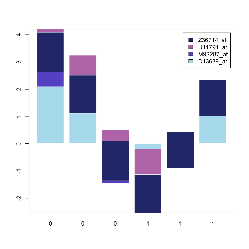 In this case the patients are indicated on the
 X axis (0 and 1 respectively)
while the gene expression level is indicate on the Y axis.
We can make some improvements to the plots.
Let’s have a look at the barplot arguments:
?barplot
We are going to focus on only a few of the histgram arguments:
beside:TRUEfor the bars to be displayed as justapoxed bars,FALSEfor stacked barshoriz:FALSEbars displayed vertically with the first bar to the left,TRUEbars are displayed horizontally with the first at the bottom.ylim,xlim: limits for the y and x axescol: colour choices
barplot(mygenelist, horiz = TRUE, col = colours, legend = TRUE,
       ylab = 'Patient', border = 'white',
        xlab = 'Gene expression level', main  = 'Cycline genes expression')
box()
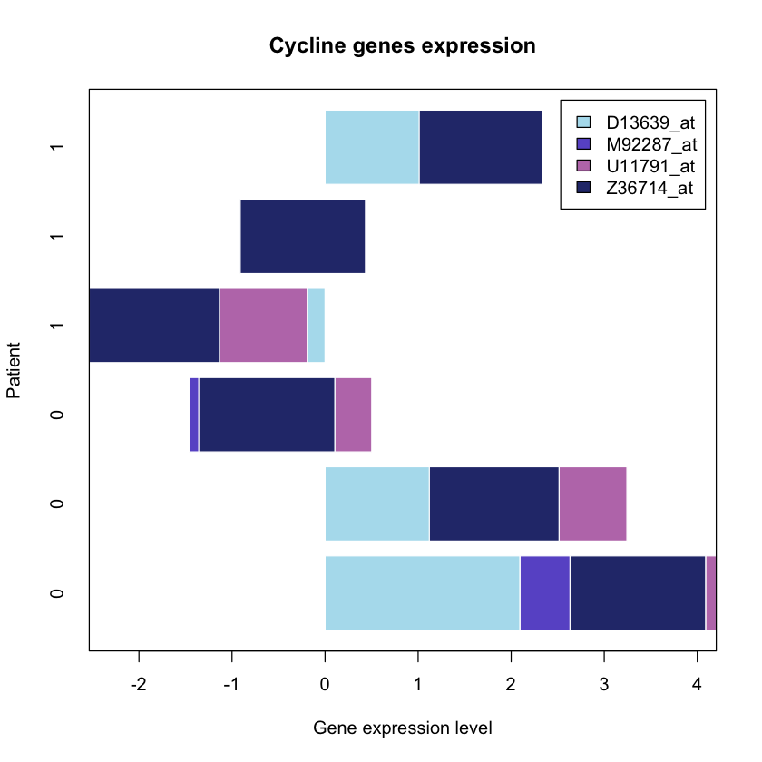 In the plot above we presented the barplots horizontally and added some colours,
which makes it easier to understand the data presented.
You can also use the barplots to represent the mean and standard error which we
will be doing in the following sections.
In the plot above we presented the barplots horizontally and added some colours,
which makes it easier to understand the data presented.
You can also use the barplots to represent the mean and standard error which we
will be doing in the following sections.
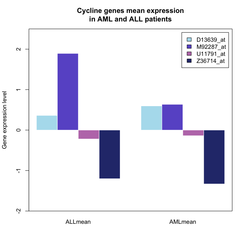
1.5. Plotting the mean
In the following we will compute the mean for the expression values of both the ALL and AML patients. We will be using the same 4 cycline genes used in the example above.
First we will compute the ALL and AML for all the patients. Once the means are computed they are combined into a single data frame.
Finally, the means are plotted using the barplot function.
# Calculating the mean of the chosen genes from patient 1 to 27 and 28 to 38
ALLmean <- rowMeans(golub[c(85,1042,1212,2240),c(1:27)])
AMLmean <- rowMeans(golub[c(85,1042,1212,2240),c(28:38)])

# Combining the mean matrices previously calculated
dataheight <- cbind(ALLmean, AMLmean)

# Plotting
barx <- barplot(dataheight, beside=T, horiz=F, col= colours, ylim=c(-2,2.5),
                legend = TRUE,border = 'white' ,
                ylab = 'Gene expression level', main = 'Cycline genes mean expression
in AML and ALL patients')
box()
1.6. Adding error bars to the previous plot
In the previous section we computed the mean expression level for 4 cycline genes between the AML and ALL patients. Sometimes it is useful to add error bars to the plots (as the one above) to convey the uncertainty in the data presented.
For such a purpose we often use the Standard Deviation:
which in turn tells us how much the values in a certain group tend to deviate from their mean value.
Let’s start calculating the Standard Deviation of the data.
In [24]:# Calculating the SD
ALLsd <- apply(golub[c(85,1042,1212,2240),c(1:27)], 1, sd)
nALL=length(c(1:27))
AMLsd <- apply(golub[c(85,1042,1212,2240),c(28:38)], 1, sd)
nAML=length(c(28:38))
# Combining the data
datasd <- cbind(ALLsd, AMLsd)
Another measure used to quantify the deviation is the standard error, which qutifies the variability in the means of our groups instead of reporting the variability among the data points.
A relatively straigtforward way to compute this is by assuming if we were to repeat a given experiment many many times, then it would roughly follow a normal distribution. Note – this is a big assumption. hence, if we assuemt hat the means follow a nosmal distribution, then the standard error (a.k.a. variability of group means) can be defined as:
which in layman terms can be read as “take the general variability of the points around their group means (the standard deviation), and scale this number by the number of points that you’ve collected”.
Since we have already computed the SD we can now compute the standard error (SE).
In [25]:datase <- cbind(ALLsd/sqrt(nALL), AMLsd/sqrt(nAML))
Now we can create a plot of the mean data as well as the SE and SD.
In [26]:# creating a panel of 2 plots displayed in 1 row
par(mfrow = c(1,2))
# Plot with the SD
datasdend<-abs(dataheight) + abs(datasd)
datasdend[c(3,4),] = - datasdend[c(3,4),]
barx <- barplot(dataheight, beside=T, horiz=F, col = colours, ylim=c(-2,2.5),
main = 'Data + SD', border = 'white')
abline(a = 0 , b = 0, h = 0)
arrows(barx, dataheight, barx, datasdend, angle=90, lwd = 2, length = 0.15,
col = 'navyblue')
box()
# Plot with the se: error associated to the mean!
datasdend<-abs(dataheight) + abs(datase)
datasdend[c(3,4),] = -datasdend[c(3,4),]
barx <- barplot(dataheight, beside=T, horiz=F, col = colours, ylim=c(-2,2.5),
main = 'Data + SE', border = 'white')
abline(a = 0 , b = 0, h = 0)
arrows(barx, dataheight, barx, datasdend, angle=90, lwd = 2, length = 0.15,
col = 'navyblue')
box()
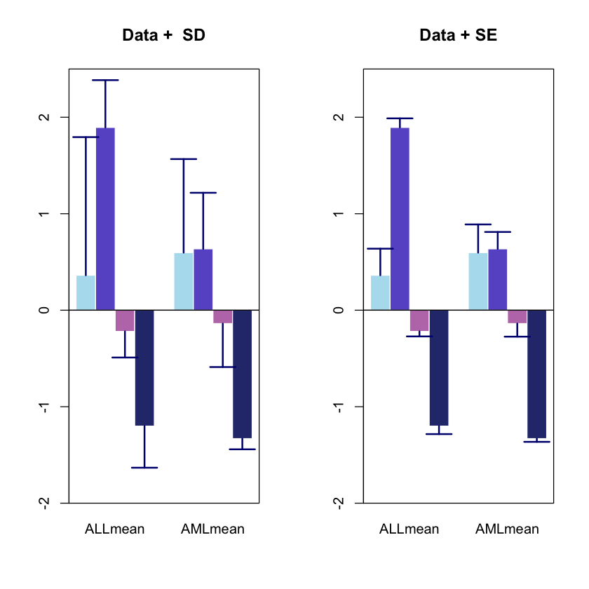 Note that the error bars for the SE are smaller than those for the SD. This is
no coincidence!
Note that the error bars for the SE are smaller than those for the SD. This is
no coincidence!
As we increase N (in the SE equation), we will decrease the error. Hence the standard error will always be smaller than the SD.
2. Data representation
This section presents some essential manners to display and visualize data.
2.1 Frequency table
Discrete data occur when the values naturally fall into categories. A frequency table simply gives the number of occurrences within a category.
A gene consists of a sequence of nucleotides (A; C; G; T)
The number of each nucleotide can be displayed in a frequency table.
This will be illustrated by the Zyxin gene which plays an important role in cell adhesion The accession number (X94991.1) of one of its variants can be found in a data base like NCBI (UniGene). The code below illustrates how to read the sequence ”X94991.1” of the species homo sapiens from GenBank, to construct a pie from a frequency table of the four nucleotides .
In [27]:library('ape')
v = read.GenBank(c("X94991.1"),as.character = TRUE)

pie(table(v$X94991.1), col = colours, border = 'white')

# prints the data as a table
table(read.GenBank(c("X94991.1"),as.character=TRUE))
  a   c   g   t
410 789 573 394 <img alt="png" src="https://trallard.github.io/Modules-template/images/notebook_images/Tutorial/Tutorial_53_1.png"/> ### 2.2 Stripcharts
An elementary method to visualize data is by using a so-called stripchart, by which the values of the data are represented as e.g. small boxes it is useful in combination with a factor that distinguishes members from different experimental conditions or patients groups.
Once again we use the CCND3 Cyclin D3 data to generate the plots.
In [30]:# data(golub, package = "multtest")
gol.fac <- factor(golub.cl,levels=0:1, labels= c("ALL","AML"))
stripchart(golub[1042,] ~ gol.fac, method = "jitter",
col = c('slateblue', 'darkgrey'), pch = 16)
 From the above figure, it can be observed that the CCND3 Cyclin D3 expression
values of the ALL patients tend to have larger expression values than those of
the AML patient.
From the above figure, it can be observed that the CCND3 Cyclin D3 expression
values of the ALL patients tend to have larger expression values than those of
the AML patient.
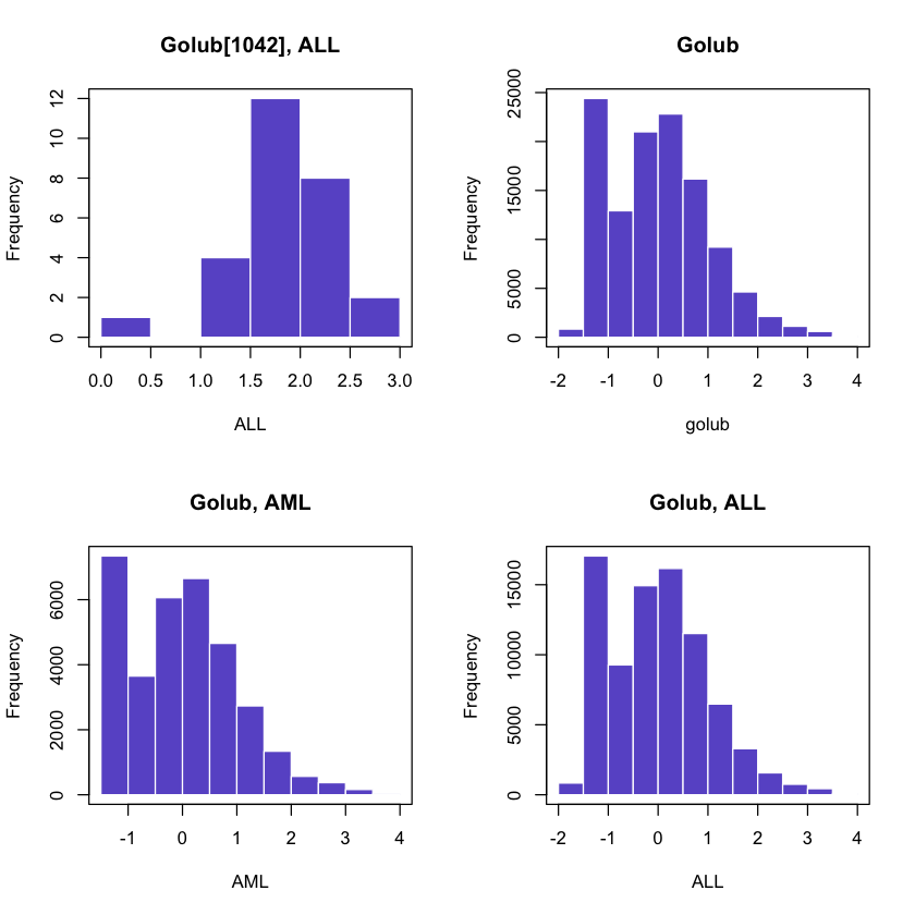
2.3 Histograms
Another method to visualize data is by dividing the range of data values into a number of intervals and to plot the frequency per interval as a bar. Such a plot is called a histogram.
We will now generate a histogram of the expression values of gene CCND3 Cyclin D3 as well as all the genes for the AML and ALL patients contained in the Golub dataset.
In [31]:par(mfrow=c(2,2))
hist(golub[1042, gol.fac == "ALL"],
col = 'slateblue', border = 'white',
main = 'Golub[1042], ALL', xlab = 'ALL')
box()
hist(golub,breaks = 10,
col = 'slateblue', border = 'white',
main = 'Golub')
box()
hist(golub[, gol.fac == "AML"],breaks = 10,
col = 'slateblue', border = 'white',
main = 'Golub, AML', xlab = 'AML')
box()
hist(golub[, gol.fac == "ALL"],breaks = 10,
col = 'slateblue', border = 'white',
main = 'Golub, ALL', xlab = 'ALL')
box()
2.3 Boxplots
A popular method to display data is by drawing a box around the 1st and the 3rd quartile (a bold line segment for the median), and the smaller line segments (whiskers) for the smallest and the largest data values.
Such a data display is known as a box-and-whisker plot.
We will start by creating a vector with gene expression values sorted in
ascending order (using the sort function).
# Sort the values of one gene
x <- sort(golub[1042, gol.fac=="ALL"], decreasing = FALSE)

# printing the first five values
x[1:5]
- 0
- 0.45827
- 0
- 1.10546
- 0
- 1.27645
- 0
- 1.32551
- 0
- 1.36844
A view on the distribution of the gene expression values of the ALL and AML
patients on gene CCND3 Cyclin D3 can be obtained by generating two separate
boxplots adjacent to each other:
# Even though we are creating two boxplots we only need one major graph
par(mfrow=c(1,1))
boxplot(golub[1042,] ~ gol.fac, col = c('lightblue2', 'mediumpurple'))
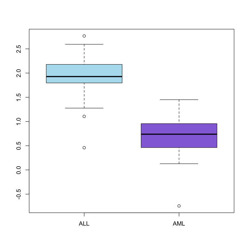 It can be observed that the gene expression values for ALL are larger than those
for AML. Furthermore, since the two sub-boxes around the median are more or less
equally wide, the data are quite symmetrically distributed around the median.
It can be observed that the gene expression values for ALL are larger than those
for AML. Furthermore, since the two sub-boxes around the median are more or less
equally wide, the data are quite symmetrically distributed around the median.
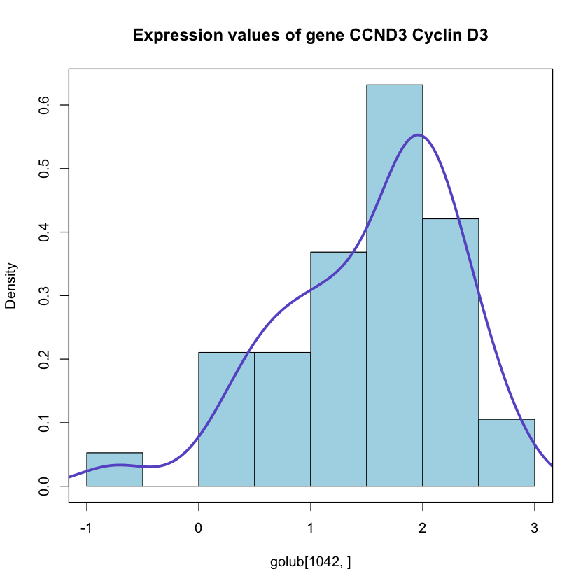
We can create a histogram of the expression values of gene CCND3 Cyclin D3 of the acute lymphoblastic leukemia patients e.g.
In [110]:hist(golub[1042,], col= 'lightblue', border= 'black', breaks= 6, freq= F,
main = 'Expression values of gene CCND3 Cyclin D3')
lines(density(golub[1042,]), col= 'slateblue', lwd = 3)
box()
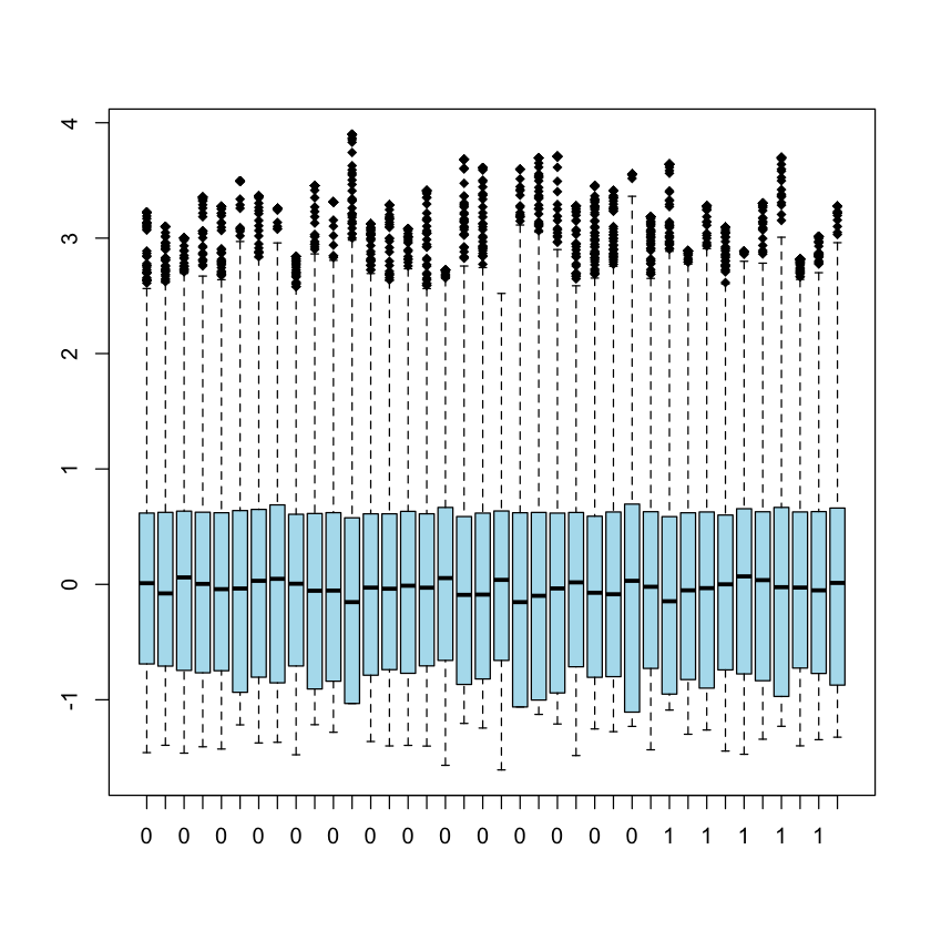
 Now we can observe the distribution of all gene expressions values in all 38
patients
Now we can observe the distribution of all gene expressions values in all 38
patients
boxplot(golub, col= 'lightblue2', lwd = 1, border="black", pch=18)
 To compute the exact values for the quartiles we need a sequence running from 0
to 1 with increments in steps of 0.25
To compute the exact values for the quartiles we need a sequence running from 0
to 1 with increments in steps of 0.25
pvec <- seq(0, 1, 0.25)
quantile(golub[1042, gol.fac=='ALL'], pvec)
- 0%
- 0.45827
- 25%
- 1.796065
- 50%
- 1.92776
- 75%
- 2.178705
- 100%
- 2.7661
Outliers are data points lying far apart from the pattern set by the majority of the data values. The implementation in R of the boxplot draws such outliers as smalle circles.
A data point x is defined (graphically, not statistically) as an outlier point
if
2.4 Q-Q plots (Quantile-quantile plots)
A method to visualize the distribution of gene expression values is y the so- called quantile-quantile (Q-Q) plots. In such a plot the quantiles of the gene expression values are displayed against the corresponding quantiles of the normal distribution (bell-shaped).
A straight line is added to represent the points which correspond exactly to the quantiles of the normal distribution. By observing the extent in which the points appear on the line, it can be evaluated to what degree the data are normally distributed. That is, the closer the gene expression values appear to the line, the more likely it is that the data are normally distributed.
To produce a Q-Q plot of the ALL gene expression values of CCND3 Cyclin D3 one may use the following.
In [116]:qqnorm(golub[1042, gol.fac == 'ALL'])
qqline(golub[1042, gol.fac == 'ALL'], col = 'slateblue', lwd = 2)
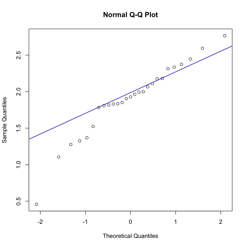 It can be seen that most of the data points are on or near the straight line,
while a few others are further away. The above example illustrates a case where
the degree of non-normality is moderate so that a clear conclusion cannot be
drawn.
It can be seen that most of the data points are on or near the straight line,
while a few others are further away. The above example illustrates a case where
the degree of non-normality is moderate so that a clear conclusion cannot be
drawn.
3. Loading tab-delimited data
In [117]:mydata<-read.delim("./NeuralStemCellData.tab.txt", row.names=1, header=T)
class(mydata)
‘data.frame’
Now try and do some exploratory analysis of your own on this data!
GvHD flow cytometry data
Only exract the CD3 positive cells
In [119]:cor(mydata[,1],mydata[,2])
plot(mydata[,1],mydata[,3])
0.956021382271511
