Classification algorithms

Random Forest implementation using sklearn

Note about the data: we will be using the famous iris data set which contains 4 variables measuring various parts of iris flowers (of 3 species) aas well as the species name.

Preliminar: load packages

In [1]:

from sklearn.datasets import load_iris
from sklearn.ensemble import RandomForestClassifier
import pandas as pd
import numpy as np

Loading the data

In [2]:

iris = load_iris()

df = pd.DataFrame(iris.data, columns=iris.feature_names)

df['species'] = pd.Categorical.from_codes(iris.target, iris.target_names)

In [3]:

df.head()

	sepal length (cm)	sepal width (cm)	petal length (cm)	petal width (cm)	species
0	5.1	3.5	1.4	0.2	setosa
1	4.9	3.0	1.4	0.2	setosa
2	4.7	3.2	1.3	0.2	setosa
3	4.6	3.1	1.5	0.2	setosa
4	5.0	3.6	1.4	0.2	setosa

Creating the training and testing data

In [4]:

df['is_train'] = np.random.uniform(0, 1, len(df)) &lt;= .75
df.head()

	sepal length (cm)	sepal width (cm)	petal length (cm)	petal width (cm)	species	is_train
0	5.1	3.5	1.4	0.2	setosa	True
1	4.9	3.0	1.4	0.2	setosa	True
2	4.7	3.2	1.3	0.2	setosa	True
3	4.6	3.1	1.5	0.2	setosa	True
4	5.0	3.6	1.4	0.2	setosa	False

In [5]:

train, test = df[df['is_train']==True], df[df['is_train']==False]

Preprocessing the data

In [6]:

# Create a list of the feature column's names
features = df.columns[:4]
features

Index(['sepal length (cm)', 'sepal width (cm)', 'petal length (cm)',
       'petal width (cm)'],
      dtype='object')

In [7]:

# train['species'] contains the actual species names. Before we can use it,
# we need to convert each species name into a digit. So, in this case there
# are three species, which have been coded as 0, 1, or 2.
y, _ = pd.factorize(train['species'])

In [8]:

print(y)

Training the random forest classifier

In [9]:

clf = RandomForestClassifier(n_jobs = 2 )

# Training the classifier
clf.fit(train[features], y)

RandomForestClassifier(bootstrap=True, class_weight=None, criterion='gini',
            max_depth=None, max_features='auto', max_leaf_nodes=None,
            min_impurity_decrease=0.0, min_impurity_split=None,
            min_samples_leaf=1, min_samples_split=2,
            min_weight_fraction_leaf=0.0, n_estimators=10, n_jobs=2,
            oob_score=False, random_state=None, verbose=0,
            warm_start=False)

Applying to the data

In [10]:

preds = iris.target_names[clf.predict(test[features])]

In [11]:

pd.crosstab(test['species'], preds, rownames=['actual'], colnames=['predicted'])

predicted	setosa	versicolor	virginica
actual
setosa	5	0	0
versicolor	0	11	0
virginica	0	2	12

View feature importance

In [12]:

list(zip(train[features], clf.feature_importances_))

[('sepal length (cm)', 0.16992592921521485),
 ('sepal width (cm)', 0.019510194239802908),
 ('petal length (cm)', 0.18115102228639413),
 ('petal width (cm)', 0.62941285425858806)]

K- Means

Preliminar : load packages

In [13]:

from sklearn.cluster import KMeans
import pandas as pd
import numpy as np
import matplotlib.pyplot as plt

%matplotlib inline

Loading the data

In [14]:

iris = load_iris()


# converting to a pandas DF for ease of use 
x = pd.DataFrame(iris.data, columns=['Sepal Length', 'Sepal Width', 'Petal Length', 'Petal Width'])
y = pd.DataFrame(iris.target, columns=['Target'])

Exploratory visualization of the data

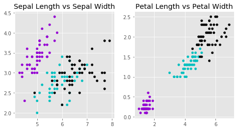
In [15]:

# creating a plot of the data first
plt.style.use('ggplot')
fig, (ax1, ax2) = plt.subplots(1, 2, figsize = (8, 4), sharey =False)
colors = np.array(['darkviolet', 'c', 'black'])

#Draw a Scatter plot for Sepal Length vs Sepal Width
#nrows=1, ncols=2, plot_number=1
ax1.scatter(x['Sepal Length'], x['Sepal Width'], c=colors[y['Target']], s = 20)
ax1.set_title('Sepal Length vs Sepal Width')

ax2.scatter(x['Petal Length'], x['Petal Width'], c= colors[y['Target']], s = 20)
ax2.set_title('Petal Length vs Petal Width');

png

Create a model object consiting of 3 clusters

In [16]:

model = KMeans(n_clusters = 3)

Apllying the model on the data

In [17]:

model.fit(x)

KMeans(algorithm='auto', copy_x=True, init='k-means++', max_iter=300,
    n_clusters=3, n_init=10, n_jobs=1, precompute_distances='auto',
    random_state=None, tol=0.0001, verbose=0)

In [18]:

# model.labels_ contains the array of cluster ids
print (model.labels_)

Visualise the output of the model

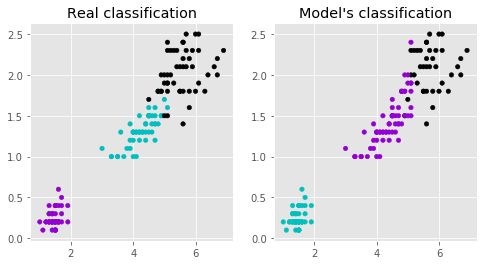
In [19]:

fig, (ax1, ax2) = plt.subplots(1, 2, figsize = (8, 4), sharey =False)

predictedY = np.choose(model.labels_, [1, 0, 2]).astype(np.int64)


# Plot the classifications that we saw earlier between Petal Length and Petal Width

ax1.scatter(x['Petal Length'], x['Petal Width'], c=colors[y['Target']], s=20)
ax1.set_title('Real classification')
 
# Plot the classifications according to the model
ax2.scatter(x['Petal Length'], x['Petal Width'], c=colors[predictedY], s=20)
ax2.set_title("Model's classification");

png

In [20]:

import time
print('This notebook was last run on: ' + time.strftime('%d/%m/%y') + ' at: ' + time.strftime('%H:%M:%S'))